4.12 t-statistics
A t-statistic is given by
\[ t = \frac{\sqrt{n} (\bar{Y} - \mu_0)}{\sqrt{\hat{V}}} \] Alternatively (from the definition of standard error), we can write
\[ t = \frac{(\bar{Y} - \mu_0)}{\textrm{s.e.}(\bar{Y})} \] though I’ll tend to use the first expression, just because I think it makes the arguments below slightly more clear.
Notice that \(t\) is something that we can calculate with our available data. \(\sqrt{n}\) is the square root of the sample size, \(\bar{Y}\) is the sample average of \(Y\), \(\mu_0\) is a number (that we have picked) coming from the null hypothesis, and \(\hat{V}\) is the sample variance of \(Y\) (e.g., computed with var(Y) in R).
Now, here is the interesting thing about t-statistics. If the null hypothesis is true, then
\[ t = \frac{\sqrt{n} (\bar{Y} - \mathbb{E}[Y])}{\sqrt{\hat{V}}} \approx \frac{\sqrt{n} (\bar{Y} - \mathbb{E}[Y])}{\sqrt{V}} \]
where we have substituted in \(\mathbb{E}[Y]\) for \(\mu_0\) (due to \(H_0\) being true) and then replaced \(\hat{V}\) with \(V\) (which holds under the law of large numbers). This is something that we can apply the CLT to, and, in particular, if \(H_0\) holds, then \[ t \rightarrow N(0,1) \] That is, if \(H_0\) is true, then \(t\) should look like a draw from a normal distribution.
Now, let’s think about what happens when the null hypothesis isn’t true. Then, we can write
\[ t = \frac{\sqrt{n} (\bar{Y} - \mu_0)}{\sqrt{\hat{V}}} \] which is just the definition of \(t\), but something different will happen here. In order for \(t\) to follow a normal distribution, we need \((\bar{Y} - \mu_0)\) to converge to 0. But \(\bar{Y}\) converges to \(\mathbb{E}[Y]\), and if the null hypothesis does not hold, then \(\mathbb{E}[Y] \neq \mu_0\) which implies that \((\bar{Y} - \mu_0) \rightarrow (\mathbb{E}[Y] - \mu_0) \neq 0\) as \(n \rightarrow \infty\). It’s still the case that \(\sqrt{n} \rightarrow \infty\). Thus, if \(H_0\) is not true, then \(t\) will diverge (recall: this means that it will either go to positive infinity or negative infinity depending on the sign of \((\mathbb{E}[Y] - \mu_0)\)).
This gives us a very good way to start to think about whether or not the data is compatible with our theory. For example, suppose that you calculate \(t\) (using your data and under your null hypothesis) and that it is equal to 1. 1 is not an “unusual” looking draw from a standard normal distribution — this suggests that you at least do not have strong evidence from data against your theory. Alternatively, suppose that you calculate that \(t=-24\). While its technically possible that you could draw \(-24\) from a standard normal distribution — it is exceedingly unlikely. We would interpret this as strong evidence against the null hypothesis, and it should probably lead you to “reject” the null hypothesis.
We have talked about some clear cases, but what about the “close calls”? Suppose you calculate that \(t=2\). Under the null hypothesis, there is about a 4.6% chance of getting a t-statistic at least this large (in absolute value). So…if \(H_0\) is true, this is a fairly unusual t-statistic, but it is not extremely unusual. What should you do?
Before we decide what to do, let’s introduce a little more terminology regarding what could go wrong with hypothesis testing. There are two ways that we could go wrong:
Type I Error — This would be to reject \(H_0\) when \(H_0\) is true
Type II Error — This would be to fail to reject \(H_0\) when \(H_0\) is false
Clearly, there is a tradeoff here. If you are really concerned with type I errors, you can be very cautious about rejecting \(H_0\). If you are very concerned about type II errors, you could aggressively reject \(H_0\). The traditional approach to trading these off in statistics is to pre-specify a significance level indicating what percentage of the time you are willing to commit a type I error. Usually the significance level is denoted by \(\alpha\) and the most common choice of \(\alpha\) is 0.05 and other common choices are \(\alpha=0.1\) or \(\alpha=0.01\). Then, good statistical tests try to make as few type II errors as possible subject to the constraint on the rate of type I errors.
Often, once you have specified a significance level, it comes with a critical value. The critical value is the value of a test statistic for which the test just rejects \(H_0\).
In practice, this leads to the following decision rule:
Reject \(H_0\) if \(|t| > c_{1-\alpha}\) where \(c_{1-\alpha}\) is the critical value corresponding to the significance level \(\alpha\).
Fail to reject \(H_0\) if \(|t| < c_{1-\alpha}\)
In our case, since \(t\) follows a normal distribution under \(H_0\), the corresponding critical value (when \(\alpha=0.05\)) is 1.96. In particular, recall what the pdf of a standard normal random variable looks like
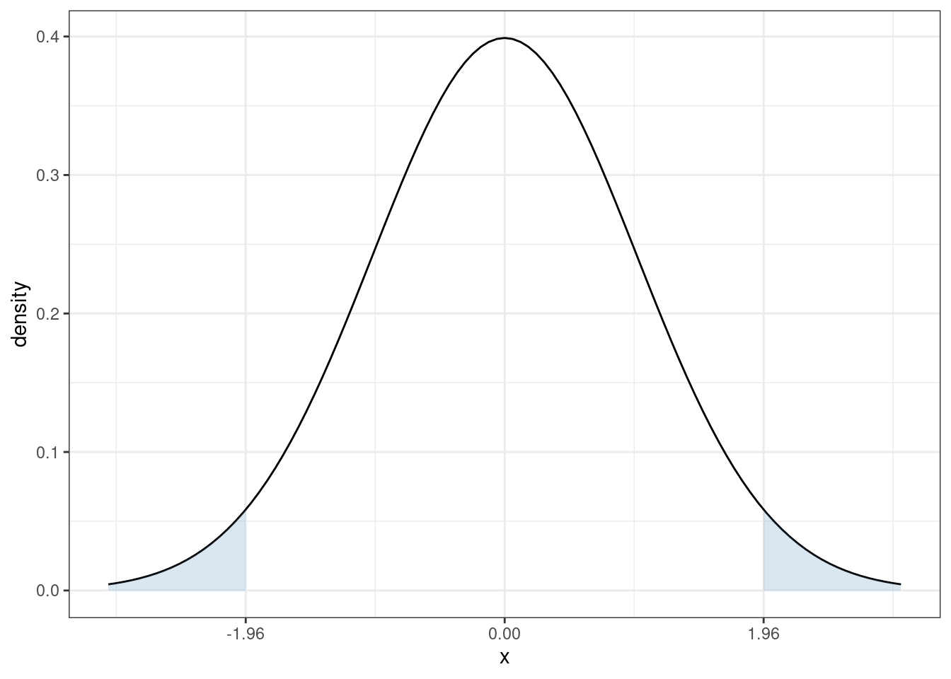
The sum of the two blue, shaded areas is 0.05. In other words, under \(H_0\), there is a 5% chance that, by chance, \(t\) would fall in the shaded areas. If you want to change the significance level, it would result in a corresponding change in the critical value so that the area in the new shaded region would adjust too. For example, if you set the significance level to be \(\alpha=0.1\), then you would need to adjust the critical value to be 1.64, and if you set \(\alpha=0.01\), then you would need to adjust the critical value to be 2.58.