3.3 pdfs, pmfs, and cdfs
SW 2.1
The distribution of a random variable describes how likely it is take on certain values.
A random variable’s distribution is fully summarized by its:
probability mass function (pmf) if the random variable is discrete
probability density function (pdf) if the random variable is continuous
The pmf is somewhat easier to explain, so let’s start there. For some discrete random variable \(X\), its pmf is given by
\[ f_X(x) = \mathrm{P}(X=x) \] That is, the probability that \(X\) takes on some particular value \(x\).
Example 3.1 Suppose that \(X\) denotes the outcome of a roll of a die. Then, \(f_X(1)\) is the probability of rolling a one. And, in particular,
\[ f_X(1) = \mathrm{P}(X=1) = \frac{1}{6} \]
Example 3.2 Let’s do a bit more realistic example where we look at the pmf of education in the U.S. Suppose that \(X\) denotes the years of education that a person has. Then, \(f_X(x)\) is the probability that a person has exactly \(x\) years of education. We can set \(x\) to different values and calculate the probabilities of a person having different amounts of education. That’s what we do in the following figure:
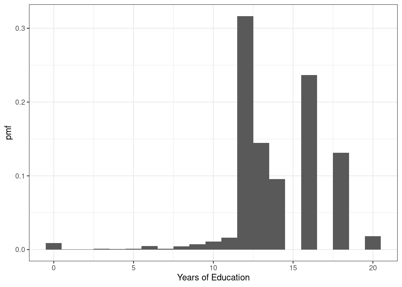
Figure 3.1: pmf of U.S. education
There are some things that are perhaps worth pointing out here. The most common amount of education in the U.S. appears to be exactly 12 years — corresponding to graduating from high school; about 32% of the population has that level of education. The next most common number of years of education is 16 — corresponding to graduating from college; about 24% of individuals have this level of education. Other relatively common values of education are 13 years (14% of individuals) and 18 (13% of individuals). About 1% of individuals report 0 years of education. It’s not clear to me whether or not that is actually true or reflects some individuals mis-reporting their education.
Before going back to the pdf, let me describe another way to fully summarize the distribution of a random variable.
- Cumulative distribution function (cdf) - The cdf of some random variable \(X\) is defined as
\[ F_X(x) = \mathrm{P}(X \leq x) \] In words, this cdf is the probability that the random \(X\) takes a value less than or equal to \(x\).
Example 3.3 Suppose \(X\) is the outcome of a roll of a die. Then, \(F_X(3) = \mathrm{P}(X \leq 3)\) is the probability of rolling 3 or lower. Thus,
\[ F_X(3) = \mathrm{P}(X \leq 3) = \frac{1}{2} \]
Example 3.4 Let’s go back to our example of years of education in the U.S. In this case, \(F_X(x)\) is the fraction of the population that has less than \(x\) years of education. We can calculate this for different values of \(x\). That’s what we do in the following figure:
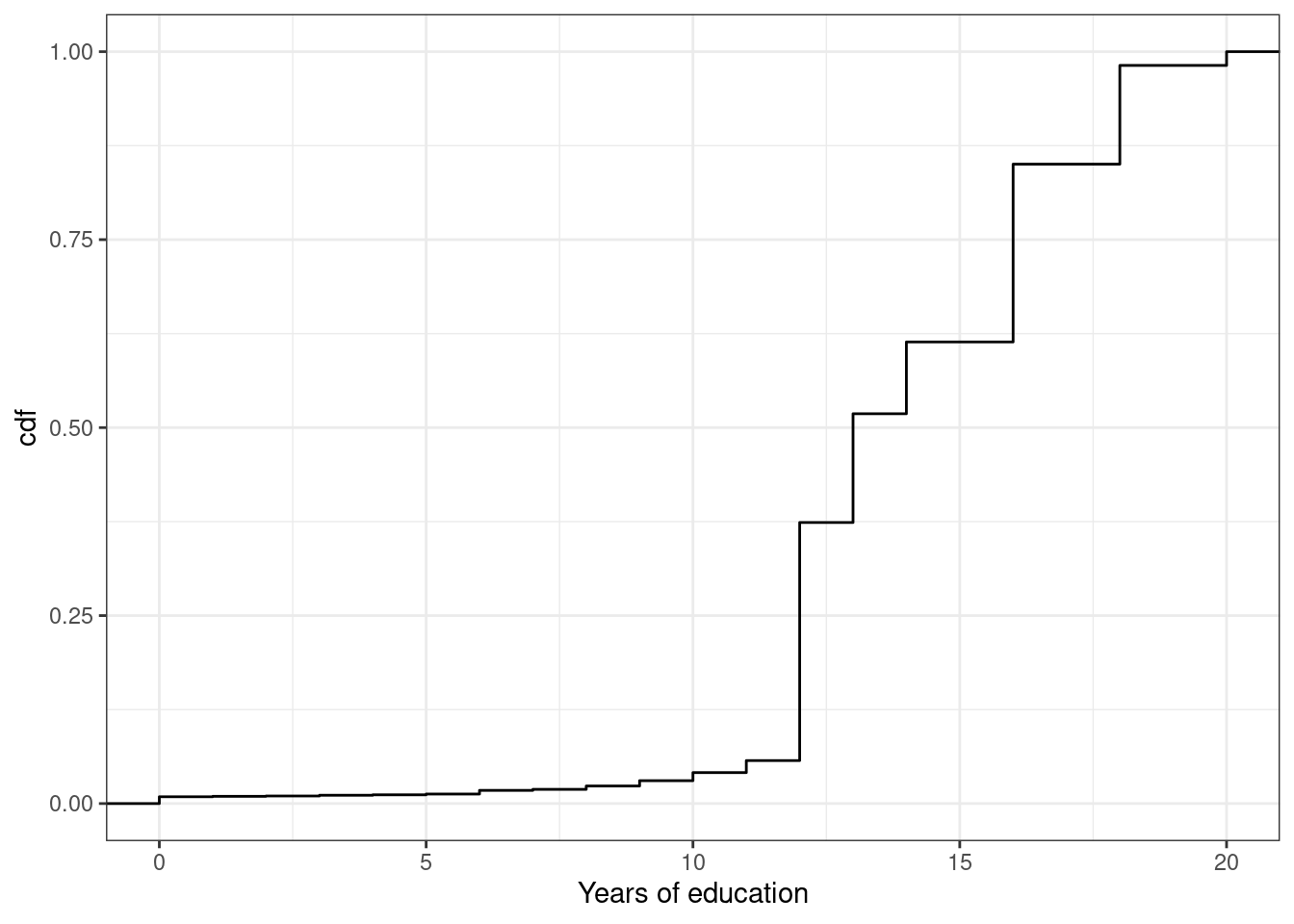
Figure 3.2: cdf of U.S. educ
You can see that the cdf is increasing in the years of education. And there are big “jumps” in the cdf at values of years of education that are common such as 12 and 16.
We’ll go over some properties of pmfs and cdfs momentarily (perhaps you can already deduce some of them from the above figures), but before we do that, we need to go over some (perhaps new) tools.