8.7 Regression Discontinuity
SW 13.4
The final type of natural experiment that we will talk about is called regression discontinuity. The sort of natural experiment is available when there is a running variable with a threshold (i.e., cutoff) where individuals above the threshold are treated while individuals below the threshold are not treated. These sorts of thresholds/cutoffs are fairly common.
Here are some examples:
Cutoffs that make students eligible for a scholarship (e.g., the Hope scholarship)
Rules about maximum numbers of students allowed in a classroom in a particular school district
Very close political elections
Very close union elections
Thresholds in tax laws
Then, the idea is to compare outcomes among individuals that “barely” were treated relative to those that “barely” weren’t treated. By construction, this often has properties that are similar to an actual experiment as those that are just above the cutoff should have observed and unobserved characteristics that are the same as those just below the cutoff.
Typically, regression discontinuity designs are implemented using a regression that includes a binary variable for participating in the treatment, the running variable itself, and the interaction between the running variable and the treatment, using only observations that are “close” to the cutoff. [What should be considered “close” to the cutoff is actually a hard choice and there are tons of papers suggesting various approaches to decide what “close” means — we’ll largely avoid this and just pick what we think is close.] The estimated coefficient on the treatment indicator variable is an estimate of the average effect of participating in the treatment among those individuals who are close to the cutoff.
This will become clearer with an example.
8.7.1 Example: Causal effect of Alcohol on Driving Deaths
In this section, we’ll be interested in the causal effect of young adult alcohol consumption on the number of deaths in car accidents.
The idea here will be to compare the number of deaths in car accidents that involve someone who is 21 or just over to the number of deaths in car accidents that involve someone who is just under 21. The reason to make this comparison is that alcohol consumption markedly increases when individuals turn 21 (due to that being the legal drinking age in the U.S.). If alcohol consumption increases car accident deaths, then we should also be able to detect a jump in the number of car accident deaths involving those who are just over 21.
The data that we have consists of age groups by age up to a particular month (agecell) and the number of car accident deaths involving that age group (mva).
library(ggplot2)
data("mlda", package="masteringmetrics")

# drop some data with missing observations
mlda <- mlda[complete.cases(mlda),]

# create treated variable
mlda$D <- 1*(mlda$agecell >= 21)
In regression discontinuity designs, it is very common to show a plot of the data. That’s what we’ll do here.
ggplot(mlda, aes(x=agecell, y=mva)) +
  geom_point() +
  geom_vline(xintercept=21) +
  xlab("age") +
  ylab("moving vehicle accident deaths") +
  theme_bw()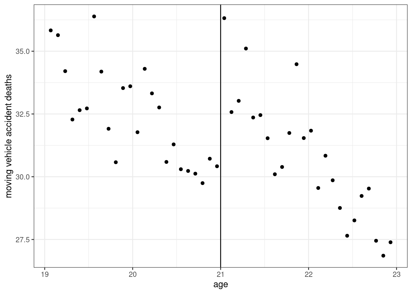
This figure at least suggests that the number of car accident deaths does appear to jump at age 21.
Now, let’s run the regression that we talked about earlier, involving a treatment dummy, age, and age interacted with the treatment.
rd_reg <- lm(mva ~ D + agecell + agecell*D, data=mlda)
summary(rd_reg)
#>
#> Call:
#> lm(formula = mva ~ D + agecell + agecell * D, data = mlda)
#>
#> Residuals:
#>     Min      1Q  Median      3Q     Max
#> -2.4124 -0.7774 -0.2913  0.8495  3.2378
#>
#> Coefficients:
#>             Estimate Std. Error t value Pr(>|t|)
#> (Intercept)  83.8492     9.3328   8.984 1.63e-11 ***
#> D            28.9450    13.8638   2.088   0.0426 *
#> agecell      -2.5676     0.4661  -5.508 1.77e-06 ***
#> D:agecell    -1.1624     0.6592  -1.763   0.0848 .
#> ---
#> Signif. codes:  0 '***' 0.001 '**' 0.01 '*' 0.05 '.' 0.1 ' ' 1
#>
#> Residual standard error: 1.299 on 44 degrees of freedom
#> Multiple R-squared:  0.7222, Adjusted R-squared:  0.7032
#> F-statistic: 38.13 on 3 and 44 DF,  p-value: 2.671e-12
These results suggest that alcohol consumption increased car accident deaths (you can see this from the estimated coefficient on D). [The setup in this example is somewhat simplified; if you wanted to be careful about how much alcohol consumption increased car accident deaths, then we would probably need to scale up our estimate by how much alcohol consumption increases on average when people turn 21. Nevertheless, what we have presented above does suggest that alcohol consumption increases car accident deaths.]
Finally, let me show one more plot that is common to report in a regression discontinuity design.
# get predicted values for plotting
mlda$preds <- predict(rd_reg)

# make plot
ggplot(mlda, aes(x=agecell, y=mva, color=as.factor(D))) +
  geom_point() +
  geom_line(aes(y=preds)) +
  geom_vline(xintercept=21) +
  labs(color="treated", x="age", y="moving vehicle accident deaths") +
  theme_bw()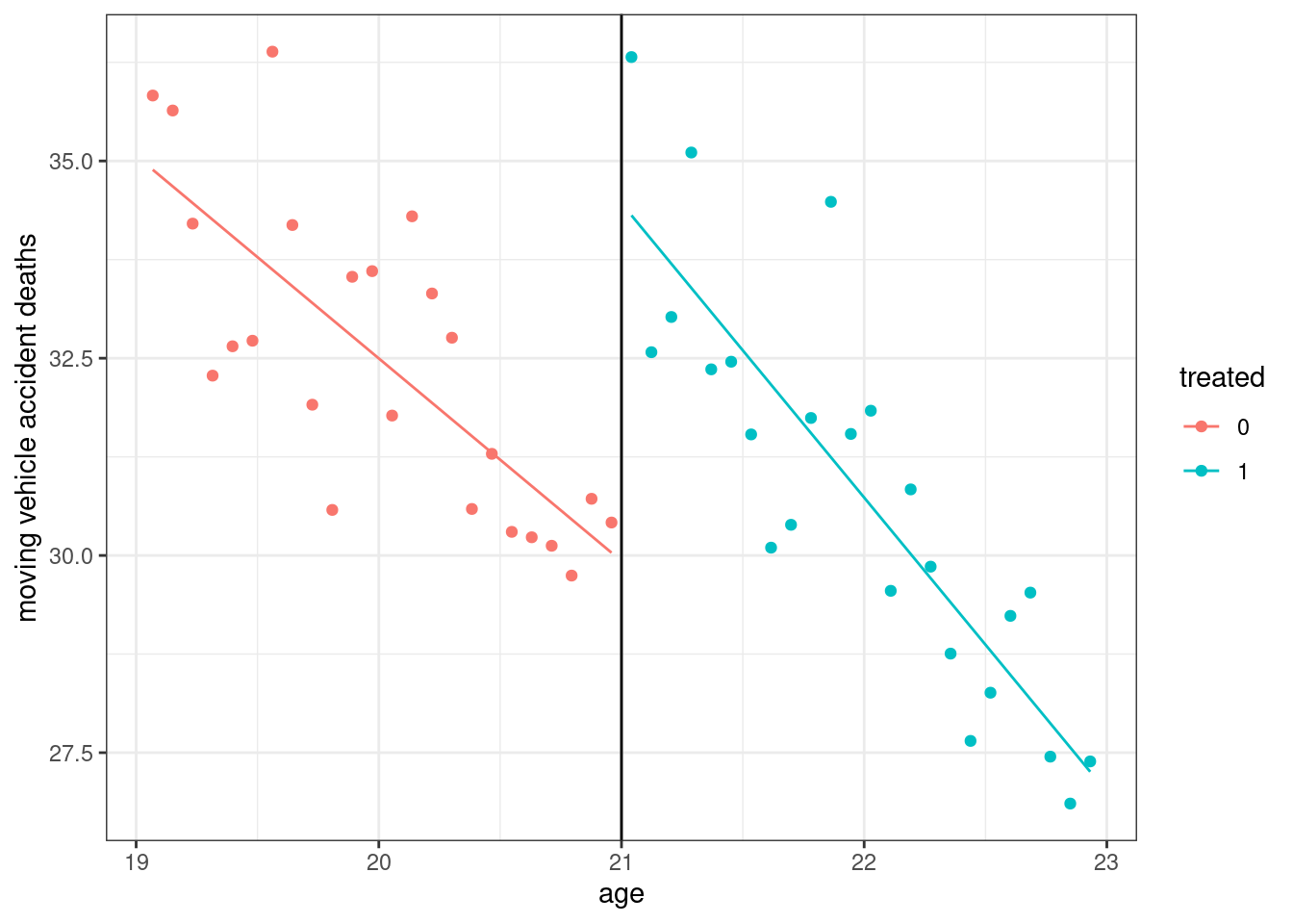
This shows the two lines that we effectively fit with the regression that included the binary variable for the treatment, the running variable, and their interaction. The “jump” between the red line and the blue line at age=21 is our estimated effect of the treatment.