4.13 P-values
Choosing a significance level is somewhat arbitrary. What did we choose 5%?
Perhaps more importantly, we are essentially throwing away a lot of information if we are to reduce the information from standard errors/t-statistics to a binary “reject” or “fail to reject”.
One alternative is to report a p-value. A p-value is the probability of observing a t-statistic as “extreme” as we did if \(H_0\) were true.
Here is an example of how to calculate a p-value. Suppose we calculate \(t=1.85\). Then,
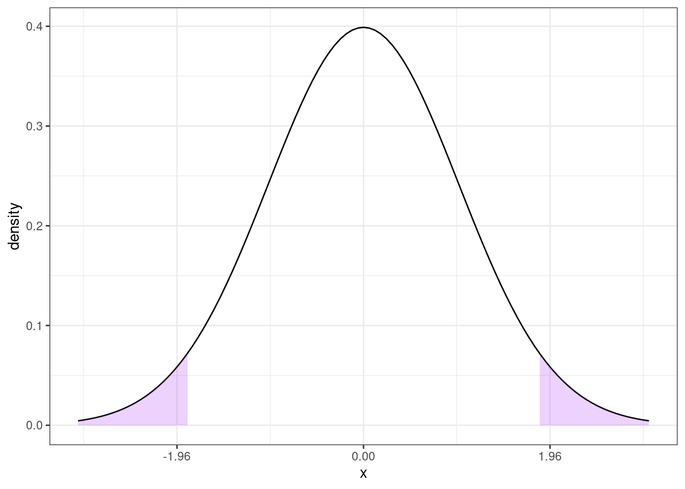
Then, under \(H_0\), the probability of getting a t-statistic “as extreme” as 1.85 corresponds to the area of the two shaded regions above. In other words, we need to to compute
\[ \textrm{p-value} = \mathrm{P}(Z \leq -1.85) + \mathrm{P}(Z \geq 1.85) \] where \(Z \sim N(0,1)\). One thing that is helpful to notice here is that, a standard normal random variable is symmetric. This means that \(\mathrm{P}(Z \leq -1.85) = \mathrm{P}(Z \geq 1.85)\). We also typically denote the cdf of a standard normal random variable with the symbol \(\Phi\). Thus,
\[
\textrm{p-value} = 2 \Phi(-1.85)
\]
I don’t know what this is off the top of my head, but it is easy to compute from a table or using R. In R, you can use the function pnorm — here, the p-value is given by 2*pnorm(-1.85) which is equal to 0.064.
More generally, if you calculate a t-statistic, \(t\), using your data and under \(H_0\), then,
\[ \textrm{p-value} = 2 \Phi(-|t|) \]