2.3 R Basics
Related Reading: IDS 2.1
In this section, we’ll start to work towards writing useful R code.
2.3.1 Objects
Related Reading: IDS 2.2
The very first step to writing code that can actually do something is to able to store things. In R, we store things in objects (perhaps sometimes I will also use the word variables).
Earlier, we used R to calculate \(1+1\). Let’s go back to the Source pane (top left pane in RStudio) and type
Press Ctrl+ENTER on this line to run it. You should see the same line down in the Console now.
Let’s think carefully about what is happening here
answeris the name of the variable (or object) that we are creating here.the
<-is the assignment operator. It means that we should assign whatever is on the right hand side of it to the variable that is on the left hand side of it1+1just computes \(1+1\) as we did earlier. Soon we will put more complicated expressions here.
You can think about the above code as computing \(1+1\) and then saving it in the variable answer.
Practice: Try creating variable called five_squared that is equal to \(5 \times 5\) (multiplication in R is done using the * symbol).
There are a number of reasons why you might like to create an object in R. Perhaps the main one is so that you can reuse it. Let’s try multiplying answer by \(3\).
If you wanted, you could also save this as its own variable too.
2.3.2 Workspace
Related Reading: IDS 2.2
Before we move on, I just want to show you what my workspace looks like now.
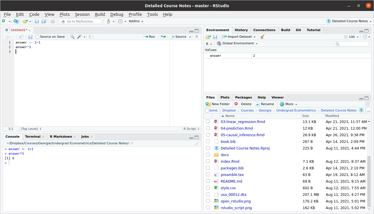
As we talked about above, you can see the code in my script in the Source pane in the top left. You can also see the code that I actually ran in the Console pane on the bottom left.
Now, take a look at the top right pane. You will see under the Environment tab that answer shows up there with a value of 2. The Environment tab keeps track of all the variables that you have created in your current session. A couple of other things that might be useful to point out there.
Later on in the class, we will often import data to work with. The “Import Dataset” button that is located in this top right pane is often useful for this.
Occasionally, you might get into the case where you have saved a bunch of variables and it would be helpful to “start over”. The broom in this pane will “clean” your workspace (this just means delete everything).
2.3.3 Importing Data
To work with actual data in R, we will need to import it. I mentioned the “Import Data” button above, but let me mention a few other possibilities here, including how to import data by writing code.
On the course website, I posted three files firm.data.csv, firm_data.RData, and firm_data.dta. All three of these contain exactly the same small, fictitious dataset, but are saved in different formats.
Probably the easiest way to import data in R is through the Files pane on the bottom right. In particular, suppose that you saved firm_data.csv in your “Downloads” folder. Try clicking the “…” (which, in the screenshot of my workspace above, is right beside the folder that I am in which is called “Detailed Course Notes”), then select your Downloads folder. This will switch the content of the Files pane to show the files in your Downloads folder. Now click firm_data.csv. This will open a menu to import the data. R is quite good at recognizing different types of data files and importing them, so this same procedure will work for firm_data.RData and firm_data.dta even though they are different types of files.
Next, let’s discuss how to import data by writing computer code (by the way, this is actually what is happening behind the scenes when you import data through the user interface as described above). “csv” stands for “Comma Separated Values”. This is basically a plain text file (e.g., try opening it in Notepad or Text Editor) where the columns are separated by commas and the rows are separated by being on different lines. Most any computer program can read this type of file; that is, you could easily import this file into, say, R, Excel, or Stata. You can import a .csv file using R code by
An RData file is the native format for saving data in R. You can import an RData file using the following command:
Similarly, a dta file the native format for saving data in Stata. You can import a dta file using the following command:
In all three cases above, what we have done is to create a new data.frame (a data.frame is a type of object that we’ll talk about in detail later on in this chapter) called firm_data that contains the data that we were trying to load.
Side Comment: The assignment operator,
<-, is a “less than sign” followed by a “hyphen”. It’s often convenient though to use the keyboard shortcutAlt+-(i.e., hold downAltand press the hypen key) to insert it. You can also use an=for assignment, but this is less commonly done in R.