3.6 Continuous Random Variables
SW 2.1
For continuous random variables, you can define the cdf in exactly the same way as we did for discrete random variables. That is, if \(X\) is a continuous random variable,
\[ F_X(x) = \mathrm{P}(X \leq x) \]
Example 3.8 Suppose \(X\) denotes an individual’s yearly wage income. The cdf of \(X\) looks like
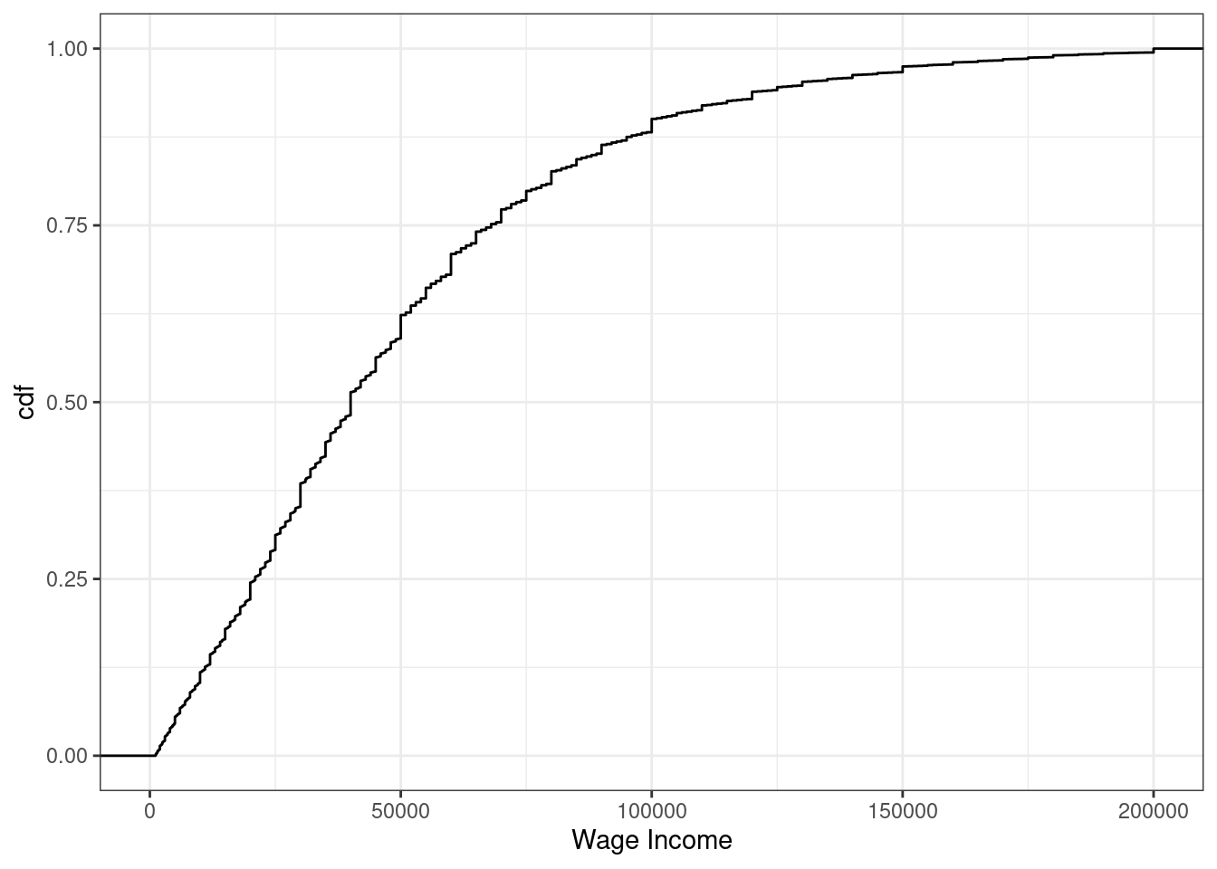
Figure 3.3: cdf of U.S. wage income
From the figure, we can see that about 24% of working individuals in the U.S. each $20,000 or less per year, 61% of working individuals earn $50,000 or less, and 88% earn $100,000 or less.
It’s trickier to define an analogue to the pmf for a continuous random variable (in fact, this is the main reason for our separate treatment of discrete and continuous random variables). For example, suppose \(X\) denotes the length of a phone conversation. As long as we can measure time finely enough, the probability that a phone conversation lasts exactly 1189.23975381 seconds (this is about 20 minutes) is 0. Instead, for a continuous random variable, we’ll define its probability density function (pdf) as the derivative of its cdf, that is,
\[ f_X(x) := \frac{d \, F_X(x)}{d \, x} \] Recall that the slope of the cdf will be larger in places where \(F_X(x)\) is “steeper”.
Regions where the pdf is larger correspond to more likely values of \(X\) — in this sense the pdf is very similar to the pmf.
We can also write the cdf as an integral over the pdf. That is,
\[ F_X(x) = \int_{-\infty}^x f_X(z) \, dz \] Integration is roughly the continuous version of a summation — thus, this expression is very similar to the expression above for the cdf in terms of the pmf when \(X\) is discrete.
More properties of cdfs
\(\mathrm{P}(X > x) = 1 - \mathrm{P}(X \leq x) = 1-F_X(x)\)
In words, if you want to calculate the probability that \(X\) is greater than some particular value \(x\), you can do that by calculating \(1-F_X(x)\).
\(\mathrm{P}(a \leq X \leq b) = F_X(b) - F_X(a)\)
In words: you can also calculate the probability that \(X\) falls in some range using the cdf.
Example 3.9 Suppose \(X\) denotes an individual’s yearly wage income. The pdf of \(X\) looks like
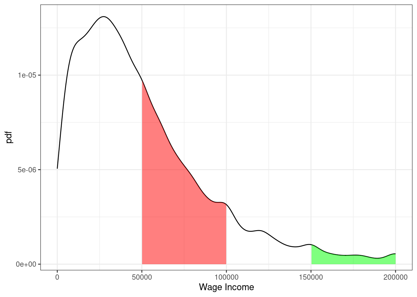
Figure 3.4: pdf of U.S. wage income
From the figure, we can see that the most common values of yearly income are around $25-30,000 per year. Notice that this corresponds to the steepest part of the cdf from the previous figure. The right tail of the distribution is also long. This means that, while incomes of $150,000+ are not common, there are some individuals who have incomes that high.
Moreover, we can use the properties of pdfs/cdfs above to calculate some specific probabilities. In particular, we can calculating probabilities by calculating integrals (i.e., regions under the curve) / relating the pdf to the cdf. First, the red region above corresponds to the probability of a person’s income being between $50,000 and $100,000. This is given by \(F(100,000) - F(50000)\). We can compute this in R using the ecdf function. In particular,
The green region in the figure is the probability of a person’s income being above $150,000. Using the above properties of cdfs, we can calculate it as \(1-F(150000)\) which is