3.16 Normal Distribution
SW 2.4
You probably learned about a lot of particular distributions of random variables in your Stats class. There are a number of important distributions:
Normal
Binomial
t-distribution
F-distribution
Chi-squared distribution
others
SW discusses a number of these distributions, and I recommend that you read/review those distributions. For us, the most important distribution is the Normal distribution [we’ll see why a few classes from now].
If a random variable \(X\) follows a normal distribution with mean \(\mu\) and variance \(\sigma^2\), we write
\[ X \sim N(\mu, \sigma^2) \] where \(\mu = \mathbb{E}[X]\) and \(\sigma^2 = \mathrm{var}(X)\).
Importantly, if we know that \(X\) follows a normal distribution, its entire distribution is fully characterized by its mean and variance. In other words, if \(X\) is normally distributed, and we also know its mean and variance, then we know everything about its distribution. [Notice that this is not generally true — if we did not know the distribution of \(X\) but knew its mean and variance, we would know two important features of the distribution of \(X\), but we would not know everything about its distribution.]
You are probably familiar with the pdf of a normal distribution — it is “bell-shaped”.
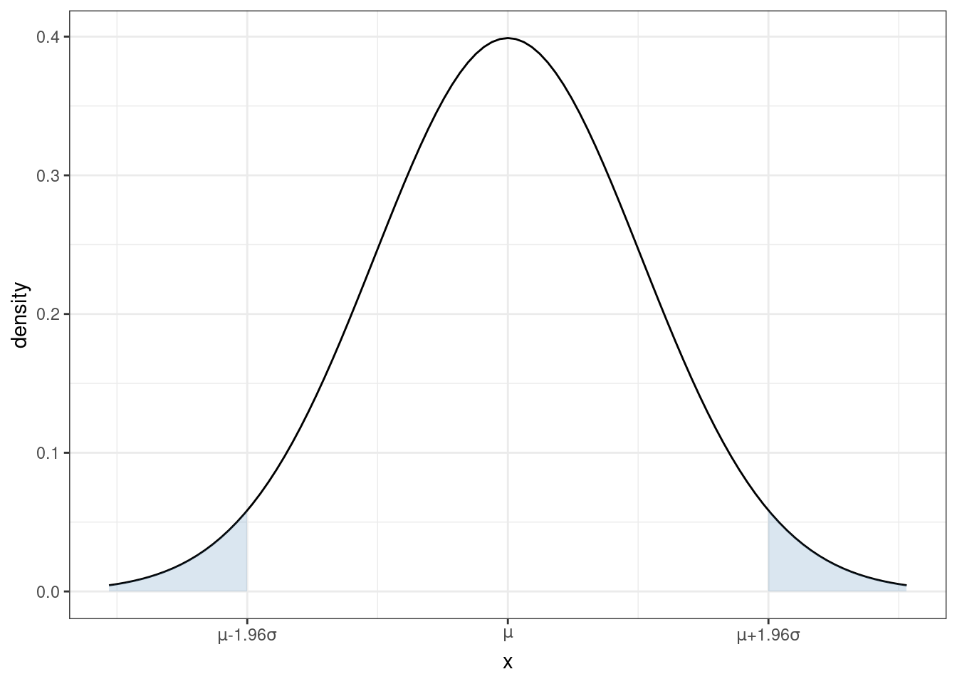
From the figure, you can see that a normal distribution is unimodal (there is just one “peak”) and symmetric (the pdf is the same if you move the same distance above \(\mu\) as when you move the same distance below \(\mu\)). This means that, for a random variable that follows a normal distribution, its median and mode are also equal to \(\mu\).
From the plot of the pdf, we can also tell that, if you make a draw from \(X \sim N(\mu,\sigma^2)\), the most likely values are near the mean. As you move further away from \(\mu\), it becomes less likely (though not impossible) for a draw of \(X\) to take that value.
Recall that we can calculate the probability that \(X\) takes on a value in a range by calculating the area under the curve of the pdf. For each shaded region in the figure, there is a 2.5% chance that \(X\) falls into that region (so the probability of \(X\) falling into either region is 5%). Another way to think about this is that there is a 95% probability that a draw of \(X\) will be in the region \([\mu-1.96\sigma, \mu+1.96\sigma]\). Later, we we talk about hypothesis testing, this will be an important property.
Earlier, we talked about standardizing random variables. If you know that a random variable follows a normal distribution, it is very common to standardize it. In particular notice that, if you create the standardized random variable
\[ Z := \frac{X - \mu}{\sigma} \quad \textrm{then} \quad Z \sim N(0,1) \] If you think back to your probability and statistics class, you may have done things like calculating a p-value by looking at a “Z-table” in the back of a textbook (I’m actually not sure if this is still commonly done because it is often easier to just do this on a computer, but, back in “my day” this was a very common exercise in statistics classes). Standardizing allows you to look at just one table for any normally distributed random variable that you could encounter rather than requiring you to have different Z table for each value of \(\mu\) and \(\sigma^2\).