Universal vs. Varying Base Period in Event Studies
Introduction
One of the main ways that researchers use our did package is to plot
event studies. These are quite useful in order to think about (i)
dynamic effects of participating in the treatment and (ii) to “pre-test”
the parallel trends assumption.
You can find an extended discussion about event studies, limitations of event study regressions in a number of relevant cases, etc. here.
This post isn’t about criticizing event study regressions; instead, what I want to talk about is the choice of the “base period” in event studies.
Types of Base Periods
Event study regressions typically have a universal base period. This means that all differences are relative to a particular period, and, most commonly, it is set to be the period immediately before the treatment starts.
In the did package, our default is to use a varying base period.
In pre-treatment periods, the base period is the immediately preceding
period; e.g., if period 4 is pre-treatment, then the base period for
this period will be period 3.
If there are violations of parallel trends in pre-treatment periods, then the interpretation of reported “effects” in pre-treatment periods in an event study differs depending on whether one uses a varying or universal base period. Here is the difference:
-
With a varying base period, the reported effects are pseudo-ATTs. They are what we would have estimated effect of participating in the treatment to be (on impact) if the treatment had occurred in that period (instead of when it actually occurred).
-
With a universal base period, event study estimates in pre-treatment periods are not themselves treatment effect parameters, but they are useful for showing how outcomes are trending over time.
In the newest version (version 2.1) of did, we have added a new
argument, base_period, to att_gt to give users the option to choose
either a varying (the default) or universal base period.
A couple of other things that are also worth mentioning:
-
In post-treatment periods, the base period is the period immediately before treatment both cases \(\implies\) the only place where this difference matters is in pre-treatment periods.
-
In pre-treatment periods, either case is just a linear combination of the other, so they essentially are just alternative ways of reporting the same information. That is, choosing between a varying or universal base period is more related to how to the “style” of presenting results and shouldn’t change conclusions about whether parallel trends is violated in pre-treatment periods, etc.
Comments/Opinions
My sense is that providing results using a varying base period tends to work better when (i) the researcher is primarily concerned with treatment effect anticipation, and/or (ii) the number of pre-treatment periods is relatively small. And that using a universal base period tends to work better when (i) the researcher thinks that there are long-term differences in trends across groups, and/or (ii) the number of pre-treatment periods is relatively large.
Finally, although using a universal based period is relatively more
common in applications, it seems to me that this is mainly because it is
easier to implement this when you are running an event study regression.
For researchers that are directly computing averages of paths of
outcomes at different lengths of exposure to the treatment (as we do in
the did package), reporting the results in using either type of base
period is easy to do.
Some Examples
Example 1: No violations of parallel trends
Let’s start with the simplest case where there are no violations of parallel trends in pre-treatment periods.
library(did) # need to load version 2.1 of package
Below is some code to generate data where parallel trends holds in all
periods, and the average effect of participating in the treatment is
equal to 1 (reset.sim and build_sim_dataset are functions in the
did package for generating simulated data).
# create data with no pre-trends
time.periods <- 5
sp <- reset.sim(time.periods=time.periods)
sp$te <- 1
data <- build_sim_dataset(sp)
data <- subset(data, G==time.periods | G==0)

# varying base period
res1_varying <- att_gt(yname="Y", xformla=~X, data=data, tname="period",
              idname="id",
              control_group="nevertreated",
              gname="G", est_method="dr")
dynamic1_varying <- aggte(res1_varying, type="dynamic")
p1_varying <- ggdid(dynamic1_varying, ylim=c(-2,2))

# universal base period
res1_universal <- att_gt(yname="Y", xformla=~X, data=data, tname="period",
              idname="id",
              control_group="nevertreated",
              gname="G", est_method="dr", base_period="universal"
              )
dynamic1_universal <- aggte(res1_universal, type="dynamic")
p1_universal <- ggdid(dynamic1_universal, ylim=c(-2,2))

ggpubr::ggarrange(p1_varying, p1_universal, nrow=1)
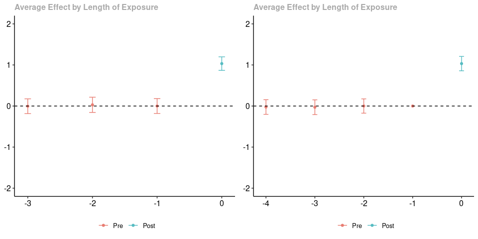
The plot on the left uses a varying base period while the plot on the right uses a universal base period. The estimated treatment effects when \(e=0\) are numerically identical. The pre-treatment estimates are not numerically identical (they are based on different paths of outcomes in pre-treatment periods for the treated group relative to the untreated group), but (as expected) neither provides any evidence against parallel trends. Finally, notice that using a varying base period provides an estimate when \(e=0\), but does not provide an estimate when \(e=-4\); using a universal base period provides an estimate when \(e=-4\) but not when \(e=-1\).
Example 2: Anticipation Effects
Next, we generate data where there anticipation effects. What is happening here is that there is a group that becomes treated in the last period and a group that never participates in the treatment (in order to not clutter the post with code, let me just point you to the complete code for this post…it is very similar to the code above). Parallel trends holds in all periods except the period right before treatment when the treated group experiences a negative “anticipation” effect of participating in the treatment.
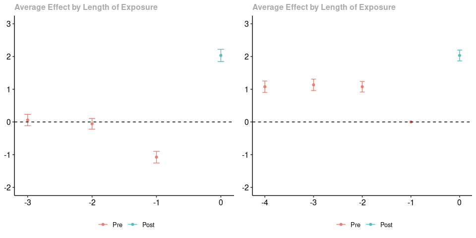
As before, the results using a varying base period are in the panel on the left, and the results using a universal base period are on the right. As before, the post-treatment estimated effects are exactly the same. To me, it seems much clearer to interpret the figure on the left (recall that there are anticipation effects that are equal to -1 in the pre-treatment period). For me, the figure on the right is hard to interpret.
Example 3: Longer Run Linear Trends
Finally, let’s consider the case where there are longish-run linear trend differences between the treated group and untreated group (and, thus, parallel trends is violated in pre-treatment periods). That is, we are in the case where, on average, outcomes are increasing by one in the treated group relative to the untreated group across all periods (both pre-treatment and post-treatment).
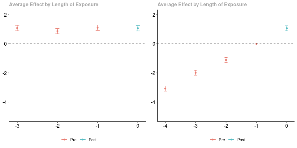
As in the earlier two cases, the panel on the left contains results using a varying base period, and the panel on the right contains results using a universal base period; likewise, the post-treatment estimates are numerically identical. In this case, to me, it seems easier to notice the linear difference in trends in the right panel. If you are careful, you can still interpret the results using a varying base period. Particularly, in every pre-treatment period, we would have over-estimated the effect of participating in the treatment (if the treatment had started in that period) – this happens because of the linear violations of parallel trends in all periods.