Is our code slow…?
I just ran into the did_imputation Stata
command which, mainly,
contains the code for implementing the ideas in Borusyak, Jaravel, and
Spiess (2021). Interestingly, the new package provides calls to recent
alternatives to two-way fixed effects in de Chaisemartin and
D’Haultfoeuille (2020), Sun and Abraham (2020), and Callaway and
Sant’Anna (2020) — so you can see estimates all in the same plot:
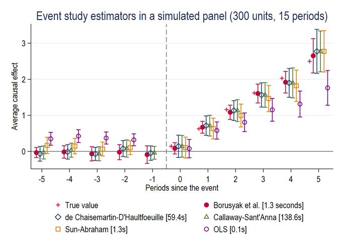
This is great, as users can display several of these new estimators along the same plot. What catches my eye here though is how slow our code appears to be: taking over two minutes to run compared to about 1 second for other approaches. This is not even a very complicated simulation either; there are 300 units and 15 time periods. If our code doesn’t run fast in this case, it is a bad sign!
The other thing that I immediately notice is that did_imputation is
written in Stata, and the main version of our code is written in R. Our
Stata version is, at the moment, a brand new proof-of-concept and still
in beta mode. Let’s see what happens if we try the same simulations but
in R using the did package instead of Stata.
Same simulations but in R
Step 1: Generate the same data
time.periods <- 15
n <- 300

# unit data
id <- 1:n
group <- sample(seq(10,16), n, replace=TRUE)
unit_data <- data.frame(id=id, group=group)

# generate panel data
panel_data <- data.frame(id=sort(rep(id,time.periods)),
                         tp=rep(rep(1:time.periods),n))
panel_data <- merge(panel_data, unit_data, by="id")
panel_data$D <- 1*(panel_data$tp >= panel_data$group)

# generate heterogeneous treatment effects by calendar date
tau <- (panel_data$D==1)*(panel_data$tp - 12.5)
panel_data$Y <- panel_data$id + 3*panel_data$tp +
  tau*panel_data$D + rnorm(nrow(panel_data))
Step 2: Use did package
For this part, let’s try two different things. First, we’ll try the default version of our code where we first compute all possible group-time average treatment effects (including pre-treatment ones), then use these to compute an event study. In addition, we default to using the multiplier bootstrap which opens up the possibility of computing uniform confidence (another default for us) that are particularly nice in the context of event studies because they provide robustness to multiple hypothesis testing (since we are estimating effects of the treatment at different lengths of exposure).
library(did)

# with 1000 bootstrap iterations
current_time <- proc.time()
out <- att_gt(yname="Y",
              gname="group",
              idname="id",
              tname="tp",
              data=panel_data,
              bstrap=TRUE,
              biters=1000)
dyn <- aggte(out, type="dynamic")
proc.time() - current_time
##    user  system elapsed
##   1.867   0.036   1.897
Second, let’s try the same thing but with analytical standard errors.
# with analytical standard errors
current_time <- proc.time()
out2 <- att_gt(yname="Y",
              gname="group",
              idname="id",
              tname="tp",
              data=panel_data,
              bstrap=FALSE)
dyn2 <- aggte(out, type="dynamic")
proc.time() - current_time
##    user  system elapsed
##   0.840   0.000   0.828
Conclusion
This seems like mostly good news. Our main code is in the R did
package, and, if you run that, our code delivers estimates of all
group-time average treatment effects and an event study (in about a
second if you use analytical standard errors) and can additionally
provide uniform confidence bands if you use the bootstrap (in about two
seconds if you use our multiplier bootstrap procedure with 1000
bootstrap iterations).
Our Stata code is slower, but we (well, mainly Fernando Rios-Avila) have been making rapid progress on the Stata implementation. At the moment, it uses a different bootstrap procedure than the R code does (which I suspect is the main reason for the differences in computational time), but I expect the Stata code to be running much faster soon.
References
-
Borusyak, Kirill, Xavier Jaravel, and Jann Spiess. “Revisiting Event Study Designs: Robust and Efficient Estimation.” Working Paper (2021).
-
Callaway, Brantly, and Pedro HC Sant’Anna. “Difference-in-differences with multiple time periods.” Journal of Econometrics (2020).
-
de Chaisemartin, Clément, and Xavier d’Haultfoeuille. “Two-way fixed effects estimators with heterogeneous treatment effects.” American Economic Review 110.9 (2020): 2964-96.
-
Sun, Liyang, and Sarah Abraham. “Estimating dynamic treatment effects in event studies with heterogeneous treatment effects.” Journal of Econometrics (2020).