Introduction to qrme: Quantile Regression with Measurement Error

Overview

The qrme package estimates quantile regression (QR) models when the dependent variable is measured with error. Classical QR applied to noisy outcomes produces biased estimates of the conditional quantile function of the true (latent) outcome. qrme() corrects this bias via a pseudo-EM algorithm that alternates between

E-step — drawing latent true outcomes given the observed noisy outcome and current QR parameters, using Metropolis–Hastings MCMC; and
M-step — re-fitting quantile regressions on the augmented data.

For the case where both the outcome and a continuous treatment variable are measured with error, see vignette("tsme-application"), which describes tsme().

A simulated example

Data-generating process

We use a location-scale DGP where the true outcome $Y^*$ depends on a uniform covariate $X$ :

$Y^* = \beta_0(U) + \beta_1(U)\,X, \quad U \sim \text{Uniform}(0,1),$

$\beta_0(u) = 1 + 3u - u^2, \qquad \beta_1(u) = e^u.$

The observed outcome is $Y = Y^* + V$ , where $V \sim N(0, \sigma_V^2)$ with $\sigma_V = 0.5$ .

library(qrme)
library(quantreg)
#> Loading required package: SparseM

n   <- 400
tau <- seq(0.10, 0.90, by = 0.10)

# true coefficient functions
b0 <- function(u) 1 + 3 * u - u^2
b1 <- function(u) exp(u)

X     <- runif(n)
U     <- runif(n)
Ystar <- b0(U) + b1(U) * X          # latent outcome
V     <- rnorm(n, sd = 0.5)         # measurement error
Y     <- Ystar + V                   # observed (noisy) outcome

dd <- data.frame(Y = Y, Ystar = Ystar, X = X)

Naive QR ignoring measurement error

Standard rq() applied to the noisy outcome is inconsistent for the QR coefficients of $Y^*$ .

fit_naive <- rq(Ystar ~ X, tau = tau, data = dd)   # infeasible truth
fit_noisy <- rq(Y     ~ X, tau = tau, data = dd)   # naive, ignores ME

# slope coefficients at each tau
rbind(
  truth  = coef(fit_naive)["X", ],
  noisy  = coef(fit_noisy)["X", ]
)
#>       tau= 0.1 tau= 0.2 tau= 0.3 tau= 0.4 tau= 0.5 tau= 0.6 tau= 0.7 tau= 0.8
#> truth 1.351121 1.471110 1.484967 1.407494 1.935130 1.869018 2.020751 2.359464
#> noisy 1.609179 1.747803 1.682019 1.641558 1.881682 1.692509 1.768411 2.266146
#>       tau= 0.9
#> truth 2.565987
#> noisy 2.525466

The naive estimates are systematically attenuated relative to the truth because additive ME compresses the conditional distribution.

ME-corrected QR with `qrme()`

qrme() takes a standard formula interface. Key arguments:

Argument	Default	Purpose
`tau`	`0.5`	quantile(s) to estimate
`n_mix`	`1`	number of Gaussian components for ME distribution
`me_distribution`	`"gaussian"`	`"gaussian"` or `"laplace"`
`mcmc_draws`	`200`	MCMC draws per E-step
`mcmc_burn_in`	`100`	burn-in draws (discarded)
`tol`	`0.01`	convergence tolerance
`max_em_iters`	`100`	maximum EM iterations
`se`	`FALSE`	compute bootstrap standard errors?
`n_boot`	`100`	bootstrap replications (if `se = TRUE`)

fit_me <- qrme(
  formula      = Y ~ X,
  data         = dd,
  tau          = tau,
  n_mix        = 1L,
  mcmc_draws   = 150L,
  mcmc_burn_in = 75L,
  tol          = 1e-2,
  max_em_iters = 30L,
  se           = FALSE,
  verbose      = FALSE
)

The result is an object of class merr. Printing it shows the estimated measurement error distribution:

print(fit_me)
#> Measurement error: gaussian
#>  Pi Mu  Sigma
#>   1  0 0.6107

Coefficient estimates

The QR coefficient matrix lives in fit_me$bet. Rows correspond to tau values; columns to regression coefficients (intercept first).

# intercept and slope at each quantile
colnames(fit_me$bet) <- c("intercept", "slope_X")
round(fit_me$bet, 3)
#>          intercept slope_X
#> tau= 0.1     1.556   1.516
#> tau= 0.2     1.647   1.575
#> tau= 0.3     1.814   1.564
#> tau= 0.4     2.017   1.617
#> tau= 0.5     2.206   1.756
#> tau= 0.6     2.319   1.956
#> tau= 0.7     2.395   2.226
#> tau= 0.8     2.454   2.437
#> tau= 0.9     2.519   2.544

Use betfun() to get a smooth interpolating function over the unit interval, which is useful for plotting the full quantile process:

bf    <- betfun(fit_me$bet, tau)
tau_g <- seq(0.10, 0.90, length.out = 200)

# betfun returns a function over scalar tau; sapply to vectorise
# coef() on a multi-tau rq object is (coefs x tau); transpose for betfun
slope_me    <- sapply(tau_g, function(u) bf(u)[2])
bf_noisy    <- betfun(t(coef(fit_noisy)), tau)
slope_noisy <- sapply(tau_g, function(u) bf_noisy(u)[2])
bf_truth    <- betfun(t(coef(fit_naive)), tau)
slope_truth <- sapply(tau_g, function(u) bf_truth(u)[2])

plot(
  tau_g, slope_me,
  type = "l", lwd = 2, col = "steelblue",
  ylim = range(slope_me, slope_noisy, slope_truth),
  xlab = expression(tau), ylab = "Slope on X",
  main = "Slope coefficient: ME-corrected vs naive vs truth"
)
lines(tau_g, slope_noisy, col = "firebrick", lwd = 2, lty = 2)
lines(tau_g, slope_truth, col = "black",     lwd = 1, lty = 3)
legend("topleft",
  legend = c("qrme (ME-corrected)", "Naive rq", "Infeasible truth"),
  col    = c("steelblue", "firebrick", "black"),
  lty    = c(1, 2, 3), lwd = c(2, 2, 1), bty = "n"
)

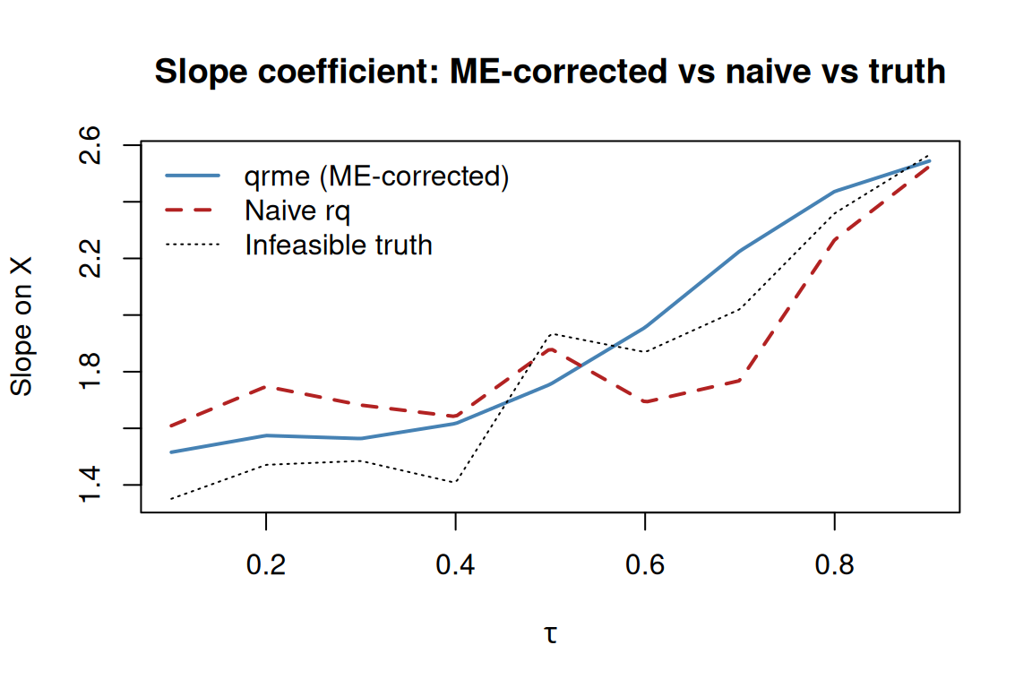
The ME-corrected estimates track the truth substantially better than the naive estimates, especially at extreme quantiles.

Recovering the measurement error distribution

The EM algorithm simultaneously estimates the ME distribution. With a single-component Gaussian specification (n_mix = 1), the estimated parameters are:

cat(sprintf(
  "ME distribution: %s\n  pi = %.3f   mu = %.3f   sigma = %.3f\n",
  fit_me$me_distribution, fit_me$pi, fit_me$mu, fit_me$sig
))
#> ME distribution: gaussian
#>   pi = 1.000   mu = 0.000   sigma = 0.611
cat("True sigma_V = 0.5\n")
#> True sigma_V = 0.5

Finite Gaussian mixtures (`n_mix > 1`)

For more flexible ME distributions, increase n_mix. With n_mix = 2 the EM fits a two-component mixture:

fit_m2 <- qrme(
  formula      = Y ~ X,
  data         = dd,
  tau          = tau,
  n_mix        = 2L,
  mcmc_draws   = 150L,
  mcmc_burn_in = 75L,
  tol          = 1e-2,
  max_em_iters = 30L,
  se           = FALSE,
  verbose      = FALSE
)
print(fit_m2)
#> Measurement error: gaussian (n_mix = 2)
#>            Pi      Mu  Sigma
#> Comp.1 0.5301 -0.5906 0.4842
#> Comp.2 0.4699  0.6664 0.3234

Model selection between mixture orders can be done via AIC() / BIC(), which call the logLik.merr() S3 method:

data.frame(
  n_mix = c(1, 2),
  AIC   = c(AIC(fit_me), AIC(fit_m2)),
  BIC   = c(BIC(fit_me), BIC(fit_m2))
)
#>   n_mix      AIC      BIC
#> 1     1 1184.047 1255.367
#> 2     2 1226.329 1315.904

Bootstrap standard errors

Set se = TRUE and choose n_boot to obtain percentile bootstrap SEs. This adds $bet_se, $sig_se, $mu_se, and $pi_se to the returned object. Bootstrap is omitted here because it is slow; a typical call looks like:

fit_se <- qrme(
  formula      = Y ~ X,
  data         = dd,
  tau          = tau,
  n_mix        = 1L,
  mcmc_draws   = 200L,
  mcmc_burn_in = 100L,
  se           = TRUE,
  n_boot       = 200L,
  n_cores      = 4L     # parallelise across bootstrap replications
)
print(fit_se)           # shows SEs alongside point estimates

Multi-start estimation

The observed-data likelihood may have multiple local optima (a property of the likelihood surface, not specific to EM), so the estimator can converge to a suboptimal solution depending on starting values. qrme_start_search() runs the estimator from multiple random starting values and returns the best fit by log-likelihood:

best <- qrme_start_search(
  formula     = Y ~ X,
  data        = dd,
  tau         = tau,
  n_starts    = 10,
  sigma_range = c(0.05, 1.5),
  n_mix       = 1L,
  mcmc_draws  = 200L
)

Summary

qrme() provides a straightforward interface for ME-corrected quantile regression. The workflow is:

Specify the model with a formula and choose tau.
Choose the ME distribution (n_mix, me_distribution).
Tune the MCMC (mcmc_draws, mcmc_burn_in, proposal_sd) and EM (tol, max_em_iters) settings.
Optionally add bootstrap SEs (se = TRUE).
Use betfun() for smooth coefficient curves and AIC()/BIC() for mixture-order selection.

For the two-sided ME extension (ME in both the outcome and a continuous treatment) see vignette("tsme-application").