\[
\newcommand{\E}{\mathbb{E}}
\renewcommand{\P}{\textrm{P}}
\let\L\relax
\newcommand{\L}{\textrm{L}} %doesn't work in .qmd, place this command at start of qmd file to use it
\newcommand{\F}{\textrm{F}}
\newcommand{\var}{\textrm{var}}
\newcommand{\cov}{\textrm{cov}}
\newcommand{\corr}{\textrm{corr}}
\newcommand{\Var}{\mathrm{Var}}
\newcommand{\Cov}{\mathrm{Cov}}
\newcommand{\Corr}{\mathrm{Corr}}
\newcommand{\sd}{\mathrm{sd}}
\newcommand{\se}{\mathrm{s.e.}}
\newcommand{\T}{T}
\newcommand{\indicator}[1]{\mathbb{1}\{#1\}}
\newcommand\independent{\perp \!\!\! \perp}
\newcommand{\N}{\mathcal{N}}
\]
11.1 Inference
SW 4.5, 5.1, 5.2, 6.6
We discussed in class the practical issues of inference in linear regression models.
These results rely on arguments building on the Central Limit Theorem (this should not surprise you as it is similar to the case for the asymptotic distribution of \(\sqrt{n}(\bar{Y} - \E[Y]))\) that we discussed earlier in the semester.
In this section, I sketch these types of arguments for you. This material is advanced, but I suggest that you study this material.
We are going to show that, in the simple linear regression model, \[\begin{align*}
\sqrt{n}(\hat{\beta}_1 - \beta_1) \rightarrow N(0,V) \quad \textrm{as} \ n \rightarrow \infty
\end{align*}\] where \[\begin{align*}
V = \frac{\E[(X-\E[X])^2 U^2]}{\var(X)^2}
\end{align*}\] and discuss how to use this result to conduct inference.
Let’s start by showing why this result holds.
To start with, recall that \[
\hat{\beta}_1 = \frac{\widehat{\cov}(X,Y)}{\widehat{\var}(X)}
\tag{11.1}\]
Before providing a main result, let’s start with noting the following:
Helpful Intermediate Result 1 Notice that \[\begin{align*}
\frac{1}{n}\sum_{i=1}^n \Big( (X_i - \bar{X})\bar{Y}\Big) &= \bar{Y} \frac{1}{n}\sum_{i=1}^n \Big( X_i-\bar{X} \Big) \\
&= \bar{Y} \left( \frac{1}{n}\sum_{i=1}^n X_i - \frac{1}{n}\sum_{i=1}^n \bar{X} \right) \\
&= \bar{Y} \Big(\bar{X} - \bar{X} \Big) \\
&= 0
\end{align*}\] where the first equality just pulls \(\bar{Y}\) out of the summation (it is a constant with respect to the summation), the second equality pushes the summation through the difference, the first part of the third equality holds by the definition of \(\bar{X}\) and the second part holds because it is an average of a constant.
This implies that \[
\frac{1}{n}\sum_{i=1}^n \Big( (X_i - \bar{X})(Y_i - \bar{Y})\Big) = \frac{1}{n}\sum_{i=1}^n \Big( (X_i - \bar{X})Y_i\Big)
\tag{11.2}\] and very similar arguments (basically the same arguments in reverse) also imply that \[
\frac{1}{n}\sum_{i=1}^n \Big( (X_i - \bar{X})X_i\Big) = \frac{1}{n}\sum_{i=1}^n \Big( (X_i - \bar{X})(X_i - \bar{X})\Big)
\tag{11.3}\] We use both Equation 11.2 and Equation 11.3 below.
Next, consider the numerator in Equation 11.1\[\begin{align*}
\widehat{\cov}(X,Y) &= \frac{1}{n} \sum_{i=1}^n (X_i - \bar{X})(Y_i - \bar{Y}) \\
&= \frac{1}{n} \sum_{i=1}^n (X_i - \bar{X})Y_i \\
&= \frac{1}{n} \sum_{i=1}^n (X_i - \bar{X})(\beta_0 + \beta_1 X_i + U_i) \\
&= \underbrace{\beta_0 \frac{1}{n} \sum_{i=1}^n (X_i - \bar{X})}_{(A)} + \underbrace{\beta_1 \frac{1}{n} \sum_{i=1}^n (X_i - \bar{X}) X_i}_{(B)} + \underbrace{\frac{1}{n} \sum_{i=1}^n (X_i - \bar{X}) U_i}_{(C)}) \\
\end{align*}\] where the first equality holds by the definition of sample covariance, the second equality holds by Equation 11.2, the third equality plugs in for \(Y_i\), and the last equality combines terms and passes the summation through the additions/subtractions.
Now, let’s consider each of these in turn.
For (A), \[\begin{align*}
\frac{1}{n} \sum_{i=1}^n X_i = \bar{X} \qquad \textrm{and} \qquad \frac{1}{n} \sum_{i=1}^n \bar{X} = \bar{X}
\end{align*}\] which implies that this term is equal to 0.
For (B), notice that \[\begin{align*}
\beta_1 \frac{1}{n} \sum_{i=1}^n (X_i - \bar{X}) X_i &= \beta_1 \frac{1}{n} \sum_{i=1}^n (X_i - \bar{X}) (X_i - \bar{X}) \\
&= \beta_1 \widehat{\var}(X)
\end{align*}\] where the first equality holds by Equation 11.3 and the second equality holds by the definition of sample variance.
For (C), well, we’ll just carry that one around for now.
Plugging in the expressions for (A), (B), and (C) back into Equation Equation 11.1 implies that \[\begin{align*}
\hat{\beta}_1 = \beta_1 + \frac{1}{n} \sum_{i=1}^n \frac{(X_i - \bar{X}) U_i}{\widehat{\var}(X)}
\end{align*}\] Next, re-arranging terms and multiplying both sides by \(\sqrt{n}\) implies that \[\begin{align*}
\sqrt{n}(\hat{\beta}_1 - \beta_1) &= \sqrt{n} \left(\frac{1}{n} \sum_{i=1}^n \frac{(X_i - \bar{X}) U_i}{\widehat{\var}(X)}\right) \\
& \approx \sqrt{n} \left(\frac{1}{n} \sum_{i=1}^n \frac{(X_i - \E[X]) U_i}{\var(X)}\right)
\end{align*}\] The last line (the approximately one) is kind of a weak argument, but basically you can replace \(\bar{X}\) and \(\widehat{\var}(X)\) and the effect of this replacement will converge to 0 in large samples (this is the reason for the approximately) — if you want a more complete explanation, sign up for my graduate econometrics class next semester.
Is this helpful? It may not be obvious, but the right hand side of the above equation is actually something that we can apply the Central Limit Theorem to. In particular, maybe it is helpful to define \(Z_i = \frac{(X_i - \E[X]) U_i}{\var(X)}\). We know that we could apply a Central Limit Theorem to \(\sqrt{n}\left( \frac{1}{n} \sum_{i=1}^n Z_i \right)\) if (i) \(Z_i\) had mean 0, and (ii) it is iid. That it is iid holds immediately from the random sampling assumption. For mean 0, \[\begin{align*}
\E[Z] &= \E\left[ \frac{(X - \E[X]) U}{\var(X)}\right] \\
&= \frac{1}{\var(X)} \E[(X - \E[X]) U] \\
&= \frac{1}{\var(X)} \E[(X - \E[X]) \underbrace{\E[U|X]}_{=0}] \\
&= 0
\end{align*}\] where the only challenging line here is the third one holds from the Law of Iterated Expectations. This means that we can apply the central limit theorem, and in particular, \(\sqrt{n} \left( \frac{1}{n} \sum_{i=1}^n Z_i \right) \rightarrow N(0,V)\) where \(V=\var(Z) = \E[Z^2]\) (where the 2nd equality here holds because \(Z\) has mean 0). Now, just substituting back in for \(Z\) implies that \[\begin{align*}
\sqrt{n}(\hat{\beta}_1 - \beta_1) \rightarrow N(0,V)
\end{align*}\] where \[
\begin{aligned}
V &= \E\left[ \left( \frac{(X - \E[X]) U}{\var(X)} \right)^2 \right] \nonumber \\
&= \E\left[ \frac{(X - \E[X])^2 U^2}{\var(X)^2}\right]
\end{aligned}
\tag{11.4}\] which is what we were aiming for.
Given this result, all our previous work on standard errors, t-statistics, p-values, and confidence intervals applies. First, let me mention the way that you would estimate \(V\) (same as always, just replace the population quantities with corresponding sample quantities).
Interestingly, these are not exactly the same as what comes from the lm command. Here’s what the difference is: R makes a simplifying assumption called “homoskedasticity” that simplifies the expression for the variance. This can result in slightly different standard errors (and therefore slightly different t-statistics, p-values, and confidence intervals too) than the ones we calculated.
An alternative package that is popular among economists for estimating regressions and getting “heteroskedasticity robust” standard errors is the estimatr package.
Call:
lm_robust(formula = mpg ~ hp, data = mtcars, se_type = "HC0")

Standard error type:  HC0

Coefficients:
            Estimate Std. Error t value  Pr(>|t|) CI Lower CI Upper DF
(Intercept) 30.09886    2.01067  14.970 1.851e-15 25.99252 34.20520 30
hp          -0.06823    0.01313  -5.196 1.338e-05 -0.09504 -0.04141 30

Multiple R-squared:  0.6024 ,   Adjusted R-squared:  0.5892
F-statistic:    27 on 1 and 30 DF,  p-value: 1.338e-05
The “HC0” standard errors are “heteroskedasticity consistent” standard errors, and you can see that they match what we calculated above.
11.2 Lab 4: Birthweight and Smoking
For this lab, we’ll use the data Birthweight_Smoking and study the relationship between infant birthweight and mother’s smoking behavior.
Run a regression of \(birthweight\) on \(smoker\). How do you interpret the results?
Use the datasummary_balance function from the modelsummary package to provide summary statistics for each variable in the data separately by smoking status of the mother. Do you notice any interesting patterns?
Now run a regression of \(birthweight\) on \(smoker\), \(educ\), \(nprevisit\), \(age\), and \(alcohol\). How do you interpret the coefficient on \(smoker\)? How does its magnitude compare to the result from #1? What do you make of this?
Now run a regression of \(birthweight\) on \(smoker\), the interaction of \(smoker\) and \(age\) and the other covariates (including \(age\)) from #3. How do you interpret the coefficient on \(smoker\) and the coefficient on the interaction term?
Now run a regression of \(birthweight\) on \(smoker\), the interaction of \(smoker\) and \(alcohol\) and the other covariates from #3. How do you interpret the coefficient on \(smoker\) and the coefficient on the interaction term?
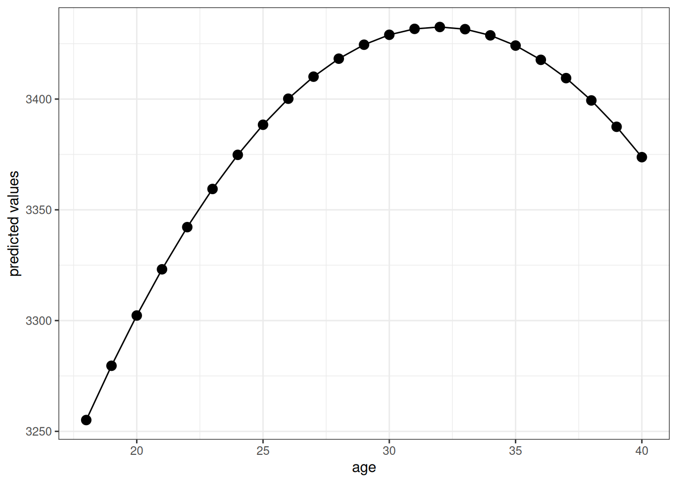
Now run a regression of \(birthweight\) on \(age\) and \(age^2\). Plot the predicted value of birthweight as a function of age for ages from 18 to 44. What do you make of this?
Now run a regression of \(\log(birthweight)\) on \(smoker\) and the other covariates from #3. How do you interpret the coefficient on \(smoker\)?
Call:
lm(formula = birthweight ~ smoker, data = Birthweight_Smoking)

Residuals:
     Min       1Q   Median       3Q      Max
-3007.06  -313.06    26.94   366.94  2322.94

Coefficients:
            Estimate Std. Error t value Pr(>|t|)
(Intercept)  3432.06      11.87 289.115   <2e-16 ***
smoker       -253.23      26.95  -9.396   <2e-16 ***
---
Signif. codes:  0 '***' 0.001 '**' 0.01 '*' 0.05 '.' 0.1 ' ' 1

Residual standard error: 583.7 on 2998 degrees of freedom
Multiple R-squared:  0.0286,    Adjusted R-squared:  0.02828
F-statistic: 88.28 on 1 and 2998 DF,  p-value: < 2.2e-16
We estimate that, on average, smoking reduces an infant’s birthweight by about 250 grams. The estimated effect is strongly statistically significant, and (I am not an expert but) that seems like a large effect of smoking to me.
# create smoker factor --- just to make table look nicerBirthweight_Smoking$smoker_factor <-as.factor(ifelse(Birthweight_Smoking$smoker==1, "smoker", "non-smoker"))datasummary_balance(~smoker_factor, data=dplyr::select(Birthweight_Smoking, -smoker),fmt=2)
non-smoker (N=2418)
smoker (N=582)
Mean
Std. Dev.
Mean
Std. Dev.
Diff. in Means
Std. Error
nprevist
11.19
3.50
10.18
4.23
-1.01
0.19
alcohol
0.01
0.11
0.05
0.22
0.04
0.01
tripre1
0.83
0.38
0.70
0.46
-0.13
0.02
tripre2
0.14
0.34
0.22
0.41
0.08
0.02
tripre3
0.03
0.16
0.06
0.24
0.04
0.01
tripre0
0.01
0.08
0.02
0.15
0.02
0.01
birthweight
3432.06
584.62
3178.83
580.01
-253.23
26.82
unmarried
0.18
0.38
0.43
0.50
0.25
0.02
educ
13.15
2.21
11.88
1.62
-1.27
0.08
age
27.27
5.37
25.32
5.06
-1.95
0.24
drinks
0.03
0.47
0.19
1.23
0.16
0.05
The things that stand out to me are:
Birthweight tends to be notably lower for smokers relative to non-smokers. The difference is about 7.4% lower birthweight for babies whose mothers smoked.
That said, smoking is also correlated with a number of other things that could be related to lower birthweights. Mothers who smoke went to fewer pre-natal visits on average, were more likely to be unmarried, were more likely to have drink alcohol during their pregnancy, were more likely to be less educated. They also were, on average, somewhat younger than mothers who did not smoke.
Call:
lm(formula = birthweight ~ smoker + educ + nprevist + age + alcohol,
    data = Birthweight_Smoking)

Residuals:
     Min       1Q   Median       3Q      Max
-2728.91  -305.26    24.69   359.63  2220.42

Coefficients:
            Estimate Std. Error t value Pr(>|t|)
(Intercept) 2924.963     74.185  39.428  < 2e-16 ***
smoker      -206.507     27.367  -7.546 5.93e-14 ***
educ           5.644      5.532   1.020    0.308
nprevist      32.979      2.914  11.318  < 2e-16 ***
age            2.360      2.178   1.083    0.279
alcohol      -39.512     76.365  -0.517    0.605
---
Signif. codes:  0 '***' 0.001 '**' 0.01 '*' 0.05 '.' 0.1 ' ' 1

Residual standard error: 570.3 on 2994 degrees of freedom
Multiple R-squared:  0.07402,   Adjusted R-squared:  0.07247
F-statistic: 47.86 on 5 and 2994 DF,  p-value: < 2.2e-16
Here we estimate that smoking reduces an infant’s birthweight by about 200 grams on average holding education, number of pre-natal visits, age, and whether or not the mother consumed alcohol constant. The magnitude of the estimated effect is somewhat smaller than the previous estimate. Due to the discussion in #2 (particularly, that smoking was correlated with a number of other characteristics that are likely associated with lower birthweights), this decrease in the magnitude is not surprising.
Call:
lm(formula = birthweight ~ smoker + I(smoker * age) + educ +
    nprevist + age + alcohol, data = Birthweight_Smoking)

Residuals:
     Min       1Q   Median       3Q      Max
-2722.56  -305.12    23.93   363.43  2244.67

Coefficients:
                Estimate Std. Error t value Pr(>|t|)
(Intercept)     2853.819     77.104  37.013  < 2e-16 ***
smoker           231.578    134.854   1.717 0.086036 .
I(smoker * age)  -17.145      5.168  -3.317 0.000919 ***
educ               4.895      5.528   0.885 0.375968
nprevist          32.482      2.913  11.151  < 2e-16 ***
age                5.528      2.375   2.328 0.019999 *
alcohol          -22.556     76.409  -0.295 0.767864
---
Signif. codes:  0 '***' 0.001 '**' 0.01 '*' 0.05 '.' 0.1 ' ' 1

Residual standard error: 569.4 on 2993 degrees of freedom
Multiple R-squared:  0.07741,   Adjusted R-squared:  0.07556
F-statistic: 41.85 on 6 and 2993 DF,  p-value: < 2.2e-16
We should be careful about the interpretatio here. We have estimated a model like
\[
\E[Birthweight|Smoker, Age, X] = \beta_0 + \beta_1 Smoker + \beta_2 Smoker \cdot Age + \cdots
\] Therefore, the partial effect of smoking is given by
\[
\E[Birthweight | Smoker=1, Age, X] - \E[Birthweight | Smoker=0, Age, X] = \beta_1 + \beta_2 Age
\] Therefore, the partial effect of smoking depends on \(Age\). For example, for \(Age=18\), the partial effect is \(\beta_1 + \beta_2 (18)\). For \(Age=25\), the partial effect is \(\beta_1 + \beta_2 (25)\), and for \(Age=35\), the partial effect is \(\beta_1 + \beta_2 (35)\). Let’s calculate the partial effect at each of those ages.
Call:
lm(formula = birthweight ~ smoker + I(smoker * alcohol) + educ +
    nprevist + age + alcohol, data = Birthweight_Smoking)

Residuals:
     Min       1Q   Median       3Q      Max
-2728.99  -304.16    24.54   359.92  2222.10

Coefficients:
                    Estimate Std. Error t value Pr(>|t|)
(Intercept)         2924.844     74.185  39.426  < 2e-16 ***
smoker              -201.852     27.765  -7.270 4.57e-13 ***
I(smoker * alcohol) -151.860    152.717  -0.994    0.320
educ                   5.612      5.532   1.014    0.310
nprevist              32.844      2.917  11.260  < 2e-16 ***
age                    2.403      2.178   1.103    0.270
alcohol               39.824    110.440   0.361    0.718
---
Signif. codes:  0 '***' 0.001 '**' 0.01 '*' 0.05 '.' 0.1 ' ' 1

Residual standard error: 570.3 on 2993 degrees of freedom
Multiple R-squared:  0.07432,   Adjusted R-squared:  0.07247
F-statistic: 40.05 on 6 and 2993 DF,  p-value: < 2.2e-16
The point estimate suggests that the effect of smoking is larger for women who consume alcohol and smoke than for women who do not drink alcohol. This seems plausible, but our evidence is not very strong here — the estimates are not statistically significant at any conventional significance level (the p-value is equal to 0.32).
reg6 <-lm(birthweight ~ age +I(age^2), data=Birthweight_Smoking)summary(reg6)
Call:
lm(formula = birthweight ~ age + I(age^2), data = Birthweight_Smoking)

Residuals:
     Min       1Q   Median       3Q      Max
-2949.81  -312.81    30.43   371.03  2452.72

Coefficients:
             Estimate Std. Error t value Pr(>|t|)
(Intercept) 2502.8949   225.6016  11.094  < 2e-16 ***
age           58.1670    16.9212   3.438 0.000595 ***
I(age^2)      -0.9099     0.3099  -2.936 0.003353 **
---
Signif. codes:  0 '***' 0.001 '**' 0.01 '*' 0.05 '.' 0.1 ' ' 1

Residual standard error: 589.6 on 2997 degrees of freedom
Multiple R-squared:  0.009261,  Adjusted R-squared:  0.0086
F-statistic: 14.01 on 2 and 2997 DF,  p-value: 8.813e-07
Call:
lm(formula = I(log(birthweight)) ~ smoker + educ + nprevist +
    age + alcohol, data = Birthweight_Smoking)

Residuals:
     Min       1Q   Median       3Q      Max
-1.96324 -0.07696  0.02435  0.12092  0.50070

Coefficients:
              Estimate Std. Error t value Pr(>|t|)
(Intercept)  7.9402678  0.0270480 293.562  < 2e-16 ***
smoker      -0.0635764  0.0099782  -6.372 2.16e-10 ***
educ         0.0022169  0.0020171   1.099    0.272
nprevist     0.0129662  0.0010624  12.205  < 2e-16 ***
age          0.0003059  0.0007941   0.385    0.700
alcohol     -0.0181053  0.0278428  -0.650    0.516
---
Signif. codes:  0 '***' 0.001 '**' 0.01 '*' 0.05 '.' 0.1 ' ' 1

Residual standard error: 0.2079 on 2994 degrees of freedom
Multiple R-squared:  0.07322,   Adjusted R-squared:  0.07167
F-statistic: 47.31 on 5 and 2994 DF,  p-value: < 2.2e-16
The estimated coefficient on \(smoker\) says that smoking during pregnancy decreases a baby’s birthweight by 6.3%, on average, holding education, number of pre-natal visits, age of the mother, and whether or not the mother consumed alcohol during the pregnancy constant.
11.4 Coding Questions
For this problem, we will use the data Caschool. This data contains information about test scores for schools from California from the 1998-1999 academic year. For this problem, we will use the variables testscr (average test score in the school), str (student teacher ratio in the school), avginc (the average income in the school district), and elpct (the percent of English learners in the school).
Run a regression of test scores on student teacher ratio, average income, and English learners percentage. Report your results. Which regressors are statistically significant? How do you know?
What is the average test score across all schools in the data?
What is the predicted average test score for a school with a student teacher ratio of 20, average income of $30,000, and 10% English learners? How does this compare to the overall average test score from part (b)?
What is the predicted average test score for a school with a student teacher ratio of 15, average income of $30,000, and 10% English learners? How does this compare to your answer from part (c)?
For this problem, we will use the data intergenerational_mobility.
Run a regression of child family income (\(child\_fincome\)) on parents’ family income (\(parent\_fincome\)). How should you interpret the estimated coefficient on parents’ family income? What is the p-value for the coefficient on parents’ family income?
Run a regression of \(\log(child\_fincome)\) on \(parent\_fincome\). How should you interpret the estimated cofficient on \(parent\_fincome\)?
Run a regression of \(child\_fincome\) on \(\log(parent\_fincome)\). How should you interpret the estimated coefficient on \(\log(parent\_fincome)\)?
Run a regression of \(\log(child\_fincome)\) on \(\log(parent\_fincome)\). How should you interpret the estimated coefficient on \(\log(parent\_fincome)\)?
For this question, we’ll use the fertilizer_2000 data.
Run a regression of \(\log(avyield)\) on \(\log(avfert)\). How do you interpret the estimated coefficient on \(\log(avfert)\)?
Now suppose that you additionally want to control for precipitation and the region that a country is located in. How would you do this? Estimate the model that you propose here, report the results, and interpret the coefficient on \(\log(avfert)\).
Now suppose that you are interested in whether the effect of fertilizer varies by region that a country is located in (while still controlling for the same covariates as in part (b)). Propose a model that can be used for this purpose. Estimate the model that you proposed, report the results, and discuss whether the effect of fertilizer appears to vary by region or not.
For this question, we will use the data mutual_funds. We’ll be interested in whether mutual funds that have higher expense ratios (these are typically actively managed funds) have higher returns relative to mutual funds that have lower expense ratios (e.g., index funds). For this problem, we will use the variables fund_return_3years, investment_type, risk_rating, size_type, fund_net_annual_expense_ratio, asset_cash, asset_stocks, asset_bonds.
Calculate the median fund_net_annual_expense_ratio.
Use the datasummary_balance function from the modelsummary package to report summary statistics for fund_return_3year, fund_net_annual_expense_ratio, risk_rating, asset_cash, asset_stocks, asset_bonds based on whether their expense ratio is above or below the median. Do you notice any interesting patterns?
Run a regression of fund_return_3years on fund_net_annual_expense_ratio. How do you interpret the results?
Now, additionally control for investment_type, risk_rating, and size_typeHint: think carefully about what type of variables each of these are and how they should enter the model. How do these results compare to the ones from part c?
Now, add the variables assets_cash, assets_stocks, and assets_bonds to the model from part d. How do you interpret these results? Compare and interpret the differences between parts c, d, and e.
For this question, we’ll use the data Lead_Mortality to study the effect of lead pipes on infant mortality in 1900.
Run a regression of infant mortality (infrate) on whether or not a city had lead pipes (lead) and interpret/discuss the results.
It turns out that the amount of lead in drinking water depends on how acidic the water is, with more acidic water leaching more of the lead (so that there is more exposure to lead with more acidic water). To measure acidity, we’ll use the pH of the water in a particular city (ph); recall that, a lower value of pH indicates higher acidity. Run a regression of infant mortality on whether or not a city has lead pipes, the pH of its water, and the interaction between having lead pipes and pH. Report your results. What is the estimated partial effect of having lead pipes from this model?
Given the results in part b, calculate an estimate of the average partial effect of having lead pipes on infant mortality.
Given the results in part b, how much does the partial effect of having lead pipes differ for cities that have a pH of 6.5 relative to a pH of 7.5?
11.5 Extra Questions
Suppose you run the following regression \[\begin{align*}
Earnings = \beta_0 + \beta_1 Education + U
\end{align*}\] with \(\E[U|Education] = 0\). How do you interpret \(\beta_1\) here?
Suppose you run the following regression \[\begin{align*}
Earnings = \beta_0 + \beta_1 Education + \beta_2 Experience + \beta_3 Female + U
\end{align*}\] with \(\E[U|Education, Experience, Female] = 0\). How do you interpret \(\beta_1\) here?
Suppose you are interested in testing whether an extra year of education increases earnings by the same amount for men and women.
Propose a regression and strategy for this sort of test.
Suppose you also want to control for experience in conducting this test, how would do it?
Suppose you run the following regression \[\begin{align*}
\log(Earnings) = \beta_0 + \beta_1 Education + \beta_2 Experience + \beta_3 Female + U
\end{align*}\] with \(\E[U|Education, Experience, Female] = 0\). How do you interpret \(\beta_1\) here?
A common extra condition (though somewhat old-fashioned) is to impose homoskedasticity. Homoskedasticity says that \(\E[U^2|X] = \sigma^2\) (i.e., the variance of the error term does not change across different values of \(X\)).
Under homoskedasticity, the expression for \(V\) in Equation 11.4 simplifies. Provide a new expression for \(V\) under homoskedasticity. Hint: you will need to use the law of iterated expectations.
Using this expression for \(V\), explain how to calculate standard errors for an estimate of \(\beta_1\) in a simple linear regression.
Explain how to construct a t-statistic for testing \(H_0: \beta_1=0\) under homoskedasticity.
Explain how to contruct a p-value for \(\beta_1\) under homoskedasticity.
Explain how to construct a 95% confidence interval for \(\beta_1\) under homoskedasticity.