Pre-Testing in a DiD Setup using the did Package
Brantly Callaway and Pedro H.C. Sant'Anna
2025-12-12
Source:vignettes/pre-testing.Rmd
pre-testing.RmdIntroduction
This vignette provides a discussion of how to conduct pre-tests in DiD setups using the did package
-
One appealing feature of many DiD applications with multiple periods is that the researcher can pre-test the parallel trends assumptions.
The idea here is simple: although one can not always test whether parallel trends itself holds, one can check if it holds in periods before treated units actually become treated.
Importantly, this is just a pre-test; it is different from an actual test. Whether or not the parallel trends assumption holds in pre-treatment periods does not actually tell you if it holds in the current period (and this is when you need it to hold!). It is certainly possible for the identifying assumptions to hold in previous periods but not hold in current periods; it is also possible for identifying assumptions to be violated in previous periods but for them to hold in current periods. That being said, we view the pre-test as a piece of evidence on the credibility of the DiD design in a particular application.
In this vignette, we demonstrate that the approach used in the did package for pre-testing may work substantially better than the more common “event study regression”.
Common Approaches to Pre-Testing in Applications
By far the most common approach to pre-testing in applications is to run an event-study regression. Here, the idea is to run a regression that includes leads and lags of the treatment dummy variable such as
where if individual has been exposed to the treatment for periods in period , and otherwise. To be clear here, it is helpful to give some examples. Suppose individual becomes treated in period 3. Then,
when and is equal to 0 in other time periods
when and is equal to 0 in other time periods
when and is equal to 0 in other time periods.
And is interpreted as the effect of treatment for different lengths of exposure to the treatment. Typically, is normalized to be equal to 0, and we follow that convention here. It is common to interpret estimated ’s with as a way to pre-test the parallel trends assumption.
Pitfalls with Event Study Regressions
Best Case Scenario for Pre-Testing
First, let’s start with a case where an event study regression is going to work well for pre-testing the parallel trends assumption
# generate dataset with 4 time periods
time.periods <- 4

# generate dynamic effects
te.e <- time.periods:1

# generate data set with these parameters
# (main thing: it generates a dataset that satisfies
# parallel trends in all periods...including pre-treatment)
data <- build_sim_dataset()

head(data)
#>       G        X id period         Y treat
#> 1     2 0.530541  1      1  4.264584     1
#> 8001  2 0.530541  1      2 10.159789     1
#> 16001 2 0.530541  1      3  9.482624     1
#> 24001 2 0.530541  1      4 10.288278     1
#> 2     4 1.123550  2      1  3.252148     1
#> 8002  4 1.123550  2      2  7.038382     1
The main thing to notice here:
- The dynamics are common across all groups. This is the case where an event-study regression will work.
Next, a bit more code
#-----------------------------------------------------------------------------
# modify the dataset a bit so that we can run an event study
#-----------------------------------------------------------------------------

# generate leads and lags of the treatment
Dtl <- sapply(-(time.periods-1):(time.periods-2), function(l) {
    dtl <- 1*( (data$period == data$G + l) & (data$G > 0) )
    dtl
})
Dtl <- as.data.frame(Dtl)
cnames1 <- paste0("Dtmin", (time.periods-1):1)
colnames(Dtl) <- c(cnames1, paste0("Dt", 0:(time.periods-2)))
data <- cbind.data.frame(data, Dtl)
row.names(data) <- NULL

head(data)
#>   G        X id period         Y treat Dtmin3 Dtmin2 Dtmin1 Dt0 Dt1 Dt2
#> 1 2 0.530541  1      1  4.264584     1      0      0      1   0   0   0
#> 2 2 0.530541  1      2 10.159789     1      0      0      0   1   0   0
#> 3 2 0.530541  1      3  9.482624     1      0      0      0   0   1   0
#> 4 2 0.530541  1      4 10.288278     1      0      0      0   0   0   1
#> 5 4 1.123550  2      1  3.252148     1      1      0      0   0   0   0
#> 6 4 1.123550  2      2  7.038382     1      0      1      0   0   0   0

#-----------------------------------------------------------------------------
# run the event study regression
#-----------------------------------------------------------------------------

# load plm package
library(plm)

# run event study regression
# normalize effect to be 0 in pre-treatment period
es <- plm(Y ~ Dtmin3 + Dtmin2 + Dt0 + Dt1 + Dt2,
          data = data, model = "within", effect = "twoways",
          index = c("id", "period"))

summary(es)
#> Twoways effects Within Model
#>
#> Call:
#> plm(formula = Y ~ Dtmin3 + Dtmin2 + Dt0 + Dt1 + Dt2, data = data,
#>     effect = "twoways", model = "within", index = c("id", "period"))
#>
#> Balanced Panel: n = 6988, T = 4, N = 27952
#>
#> Residuals:
#>       Min.    1st Qu.     Median    3rd Qu.       Max.
#> -9.8577453 -0.7594999  0.0066022  0.7639995 11.6570179
#>
#> Coefficients:
#>        Estimate Std. Error t-value Pr(>|t|)
#> Dtmin3 0.041851   0.070134  0.5967   0.5507
#> Dtmin2 0.023539   0.050044  0.4704   0.6381
#> Dt0    4.012515   0.043824 91.5602   <2e-16 ***
#> Dt1    3.005615   0.054473 55.1767   <2e-16 ***
#> Dt2    2.098672   0.077281 27.1565   <2e-16 ***
#> ---
#> Signif. codes:  0 '***' 0.001 '**' 0.01 '*' 0.05 '.' 0.1 ' ' 1
#>
#> Total Sum of Squares:    82617
#> Residual Sum of Squares: 55795
#> R-Squared:      0.32466
#> Adj. R-Squared: 0.099232
#> F-statistic: 2014.84 on 5 and 20956 DF, p-value: < 2.22e-16

#-----------------------------------------------------------------------------
# make an event study plot
#-----------------------------------------------------------------------------

# some housekeeping for making the plot
# add 0 at event time -1
coefs1 <- coef(es)
ses1 <- sqrt(diag(summary(es)$vcov))
idx.pre <- 1:(time.periods-2)
idx.post <- (time.periods-1):length(coefs1)
coefs <- c(coefs1[idx.pre], 0, coefs1[idx.post])
ses <- c(ses1[idx.pre], 0, ses1[idx.post])
exposure <- -(time.periods-1):(time.periods-2)

cmat <- data.frame(coefs=coefs, ses=ses, exposure=exposure)

library(ggplot2)

ggplot(data = cmat, mapping = aes(y = coefs, x = exposure)) +
  geom_line(linetype = "dashed") +
  geom_point() +
  geom_errorbar(aes(ymin = (coefs-1.96*ses), ymax = (coefs+1.96*ses)), width = 0.2) +
  ylim(c(-2, 5)) +
  theme_bw()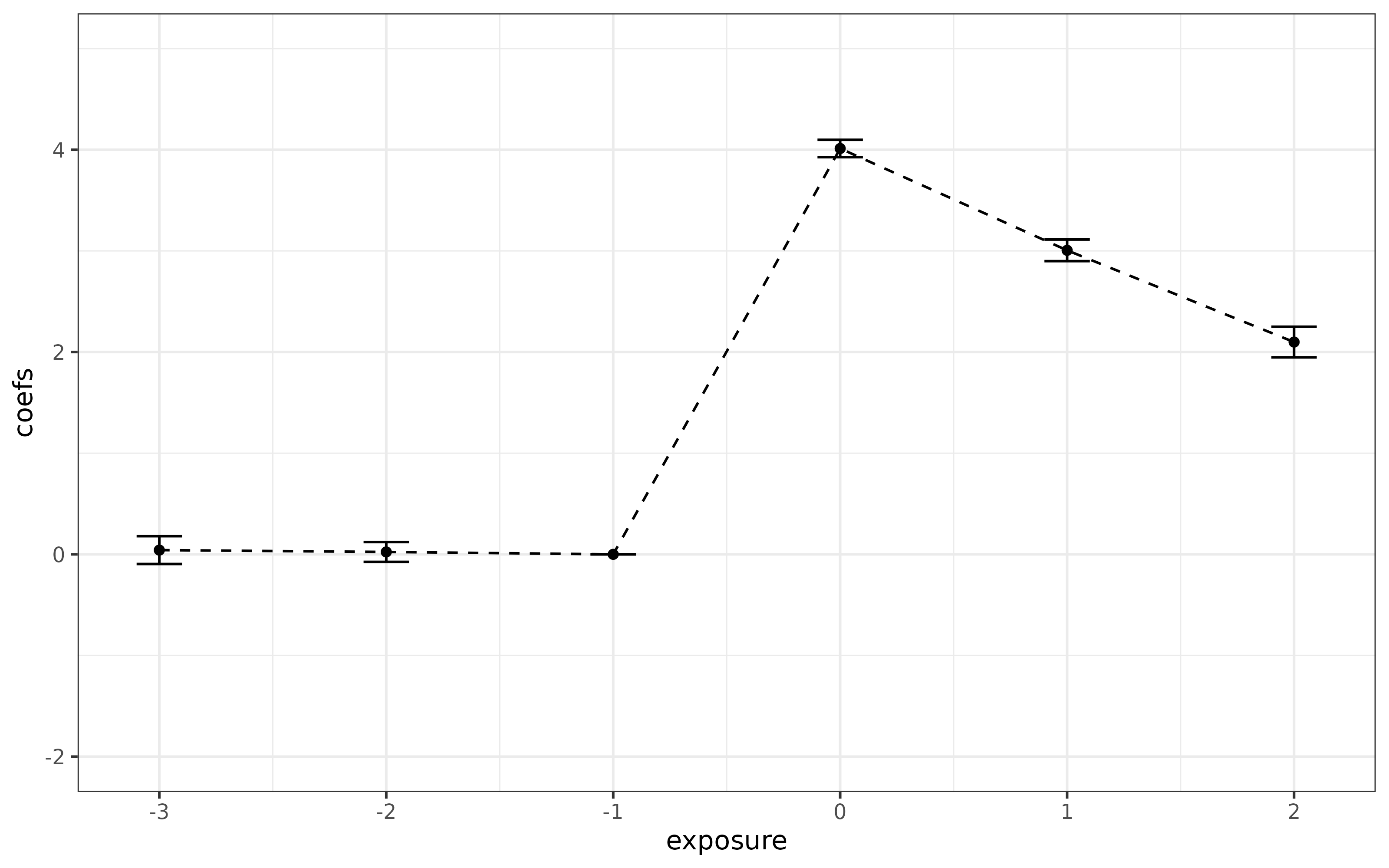
You will notice that everything looks good here. The pre-test performs well (the caveat to this is that the standard errors are “pointwise” and would be better to have uniform confidence bands though this does not seem to be standard practice in applications).
We can compare this to what happens using the did
package:
# estimate group-group time average treatment effects
did_att_gt <- att_gt(yname = "Y",
                     tname = "period",
                     idname = "id",
                     gname = "G",
                     data = data,
                     bstrap = FALSE,
                     cband = FALSE)
summary(did_att_gt)
#>
#> Call:
#> att_gt(yname = "Y", tname = "period", idname = "id", gname = "G",
#>     data = data, bstrap = FALSE, cband = FALSE)
#>
#> Reference: Callaway, Brantly and Pedro H.C. Sant'Anna.  "Difference-in-Differences with Multiple Time Periods." Journal of Econometrics, Vol. 225, No. 2, pp. 200-230, 2021. <https://doi.org/10.1016/j.jeconom.2020.12.001>, <https://arxiv.org/abs/1803.09015>
#>
#> Group-Time Average Treatment Effects:
#>  Group Time ATT(g,t) Std. Error [95% Pointwise  Conf. Band]
#>      2    2   4.0048     0.0859          3.8364      4.1732 *
#>      2    3   3.0652     0.1129          2.8438      3.2865 *
#>      2    4   2.1123     0.1466          1.8249      2.3997 *
#>      3    2  -0.0276     0.0491         -0.1237      0.0685
#>      3    3   3.9993     0.1033          3.7968      4.2018 *
#>      3    4   2.9554     0.1315          2.6976      3.2132 *
#>      4    2  -0.0420     0.0516         -0.1433      0.0592
#>      4    3   0.0016     0.0491         -0.0946      0.0977
#>      4    4   4.0304     0.1369          3.7620      4.2988 *
#> ---
#> Signif. codes: `*' confidence band does not cover 0
#>
#> P-value for pre-test of parallel trends assumption:  0.79239
#> Control Group:  Never Treated,  Anticipation Periods:  0
#> Estimation Method:  Doubly Robust

# plot them
ggdid(did_att_gt)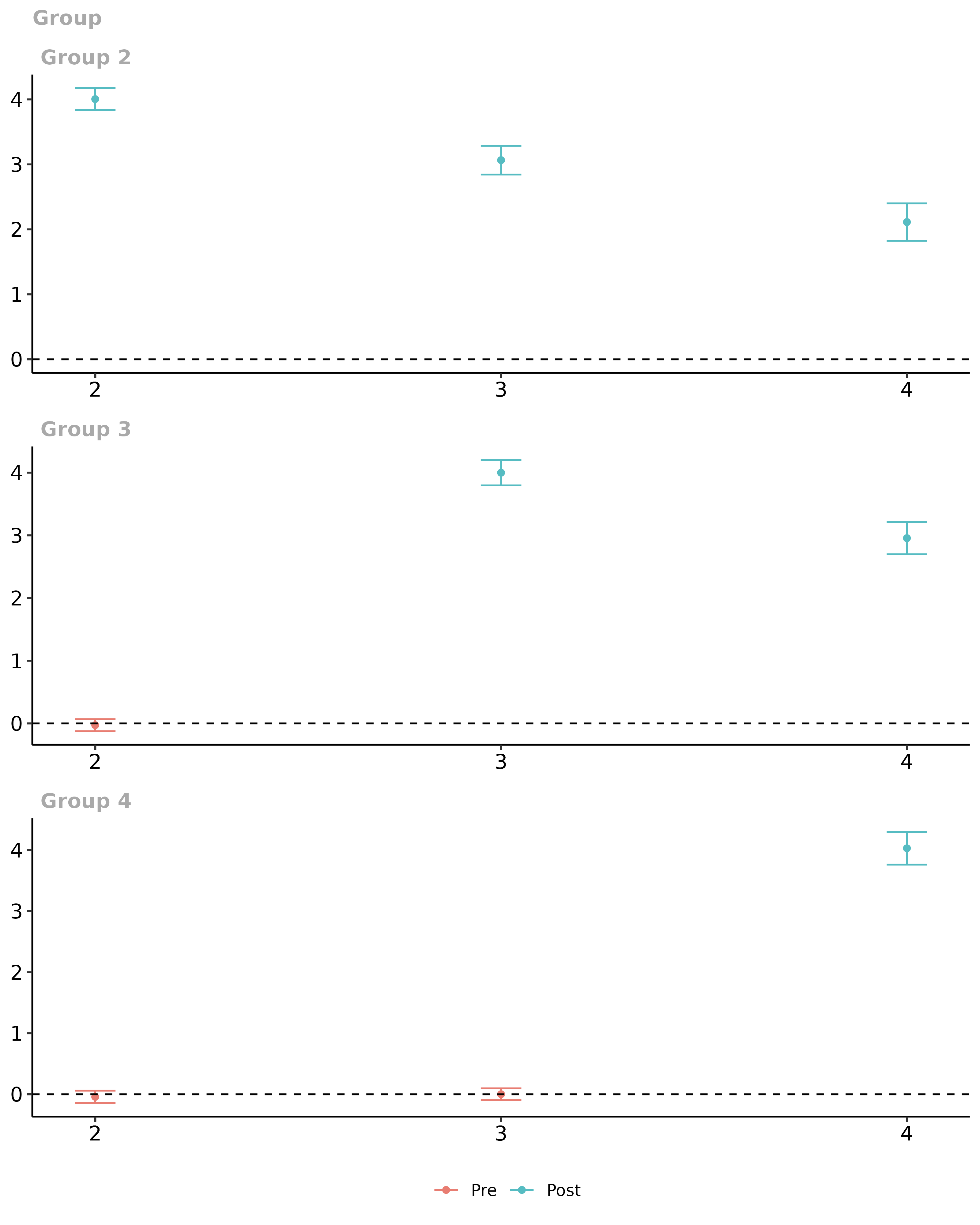
# aggregate them into event study plot
did_es <- aggte(did_att_gt, type = "dynamic")

# plot the event study
ggdid(did_es)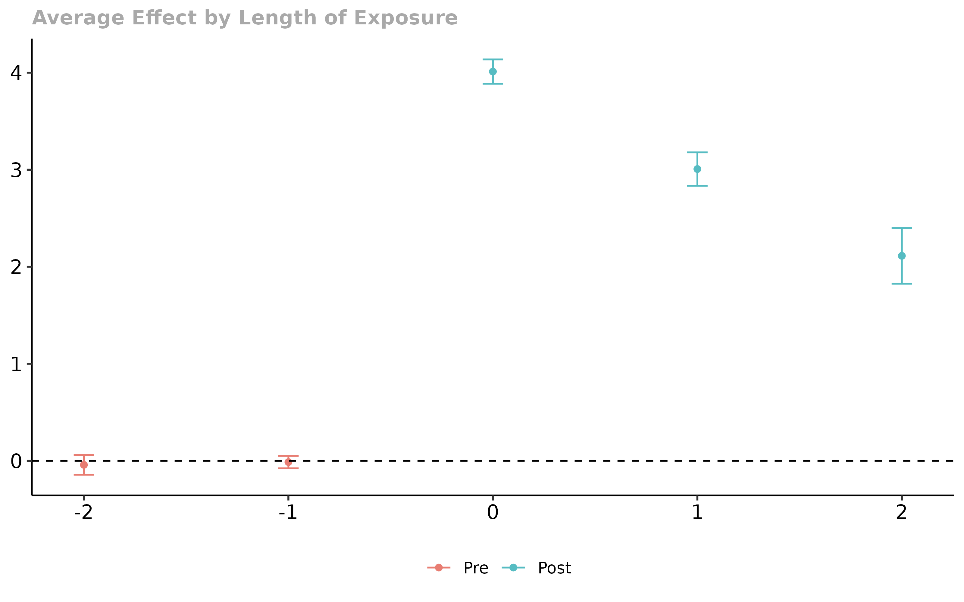
Overall, everything looks good using either approach. (Just to keep
things fair, we report pointwise confidence intervals for group-time
average treatment effects, but it is easy to get uniform confidence
bands by setting the options bstrap=TRUE, cband=TRUE to the
call to att_gt.)
Pitfall: Selective Treatment Timing
Sun and Abraham (2021) point out a major limitation of event study regressions: when there is selective treatment timing the end up being weighted averages of treatment effects across different lengths of exposures.
Selective treatment timing means that individuals in different groups experience systematically different effects of participating in the treatment from individuals in other groups. For example, there would be selective treatment timing if individuals choose to be treated in earlier periods if they tend to experience larger benefits from participating in the treatment. This sort of selective treatment timing is likely to be present in many applications in economics / policy evaluation.
Contrary to event study regressions, pre-tests based on group-time average treatment effects (or based on group-time average treatment effects that are aggregated into an event study plot) are still valid even in the presence of selective treatment timing.
To see this in action, let’s keep the same example as before, but add selective treatment timing.
# generate dataset with 4 time periods
time.periods <- 4

# generate dynamic effects
te.e <- time.periods:1

# generate selective treatment timing
# (*** this is what is different here ***)
te.bet.ind <- time.periods:1 / (time.periods/2)

# generate data set with these parameters
# (main thing: it generates a dataset that satisfies
# parallel trends in all periods...including pre-treatment)
data <- build_sim_dataset()
# run through same code as in earlier example...omitted
# run event study regression
# normalize effect to be 0 in pre-treatment period
es <- plm(Y ~ Dtmin3 + Dtmin2 + Dt0 + Dt1 + Dt2,
          data = data, model = "within", effect = "twoways",
          index = c("id", "period"))

summary(es)
#> Twoways effects Within Model
#>
#> Call:
#> plm(formula = Y ~ Dtmin3 + Dtmin2 + Dt0 + Dt1 + Dt2, data = data,
#>     effect = "twoways", model = "within", index = c("id", "period"))
#>
#> Balanced Panel: n = 6988, T = 4, N = 27952
#>
#> Residuals:
#>       Min.    1st Qu.     Median    3rd Qu.       Max.
#> -10.158205  -0.751216   0.023376   0.805780  11.190180
#>
#> Coefficients:
#>        Estimate Std. Error t-value  Pr(>|t|)
#> Dtmin3 0.938180   0.071538 13.1144 < 2.2e-16 ***
#> Dtmin2 0.424155   0.051047  8.3092 < 2.2e-16 ***
#> Dt0    3.655215   0.044701 81.7695 < 2.2e-16 ***
#> Dt1    3.199891   0.055563 57.5898 < 2.2e-16 ***
#> Dt2    2.610583   0.078828 33.1173 < 2.2e-16 ***
#> ---
#> Signif. codes:  0 '***' 0.001 '**' 0.01 '*' 0.05 '.' 0.1 ' ' 1
#>
#> Total Sum of Squares:    79441
#> Residual Sum of Squares: 58052
#> R-Squared:      0.26925
#> Adj. R-Squared: 0.025329
#> F-statistic: 1544.28 on 5 and 20956 DF, p-value: < 2.22e-16
# run through same code as before...omitted

# new event study plot
ggplot(data = cmat, mapping = aes(y = coefs, x = exposure)) +
  geom_line(linetype = "dashed") +
  geom_point() +
  geom_errorbar(aes(ymin = (coefs-1.96*ses), ymax = (coefs+1.96*ses)), width = 0.2) +
  ylim(c(-2, 5)) +
  theme_bw()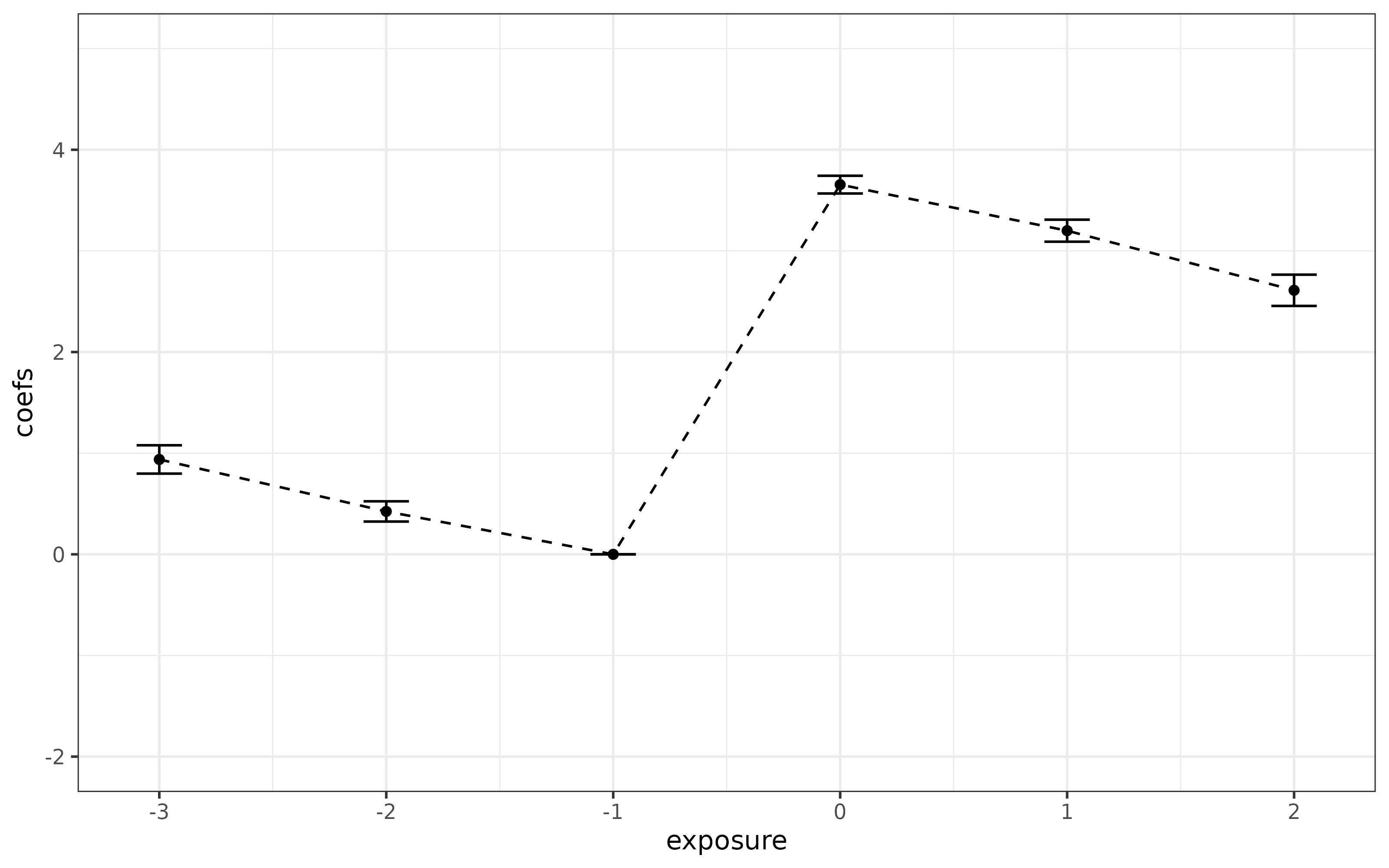
In contrast to the last case, it is clear that things have gone wrong here. Parallel trends holds in all time periods and for all groups here, but the event study regression incorrectly rejects that parallel trends holds – this is due to the selective treatment timing.
We can compare this to what happens using the did
package:
# estimate group-group time average treatment effects
did.att.gt <- att_gt(yname = "Y",
                     tname = "period",
                     idnam = "id",
                     gname = "G",
                     data = data
                     )
summary(did.att.gt)
#>
#> Call:
#> att_gt(yname = "Y", tname = "period", idname = "id", gname = "G",
#>     data = data)
#>
#> Reference: Callaway, Brantly and Pedro H.C. Sant'Anna.  "Difference-in-Differences with Multiple Time Periods." Journal of Econometrics, Vol. 225, No. 2, pp. 200-230, 2021. <https://doi.org/10.1016/j.jeconom.2020.12.001>, <https://arxiv.org/abs/1803.09015>
#>
#> Group-Time Average Treatment Effects:
#>  Group Time ATT(g,t) Std. Error [95% Simult.  Conf. Band]
#>      2    2   5.0030     0.0868        4.7636      5.2423 *
#>      2    3   4.0634     0.1104        3.7590      4.3677 *
#>      2    4   3.1105     0.1424        2.7180      3.5029 *
#>      3    2  -0.0276     0.0497       -0.1646      0.1095
#>      3    3   3.9993     0.1069        3.7047      4.2939 *
#>      3    4   2.9554     0.1323        2.5909      3.3200 *
#>      4    2  -0.0420     0.0511       -0.1828      0.0987
#>      4    3   0.0016     0.0493       -0.1343      0.1374
#>      4    4   2.0335     0.1396        1.6487      2.4182 *
#> ---
#> Signif. codes: `*' confidence band does not cover 0
#>
#> P-value for pre-test of parallel trends assumption:  0.79239
#> Control Group:  Never Treated,  Anticipation Periods:  0
#> Estimation Method:  Doubly Robust

# plot them
ggdid(did.att.gt)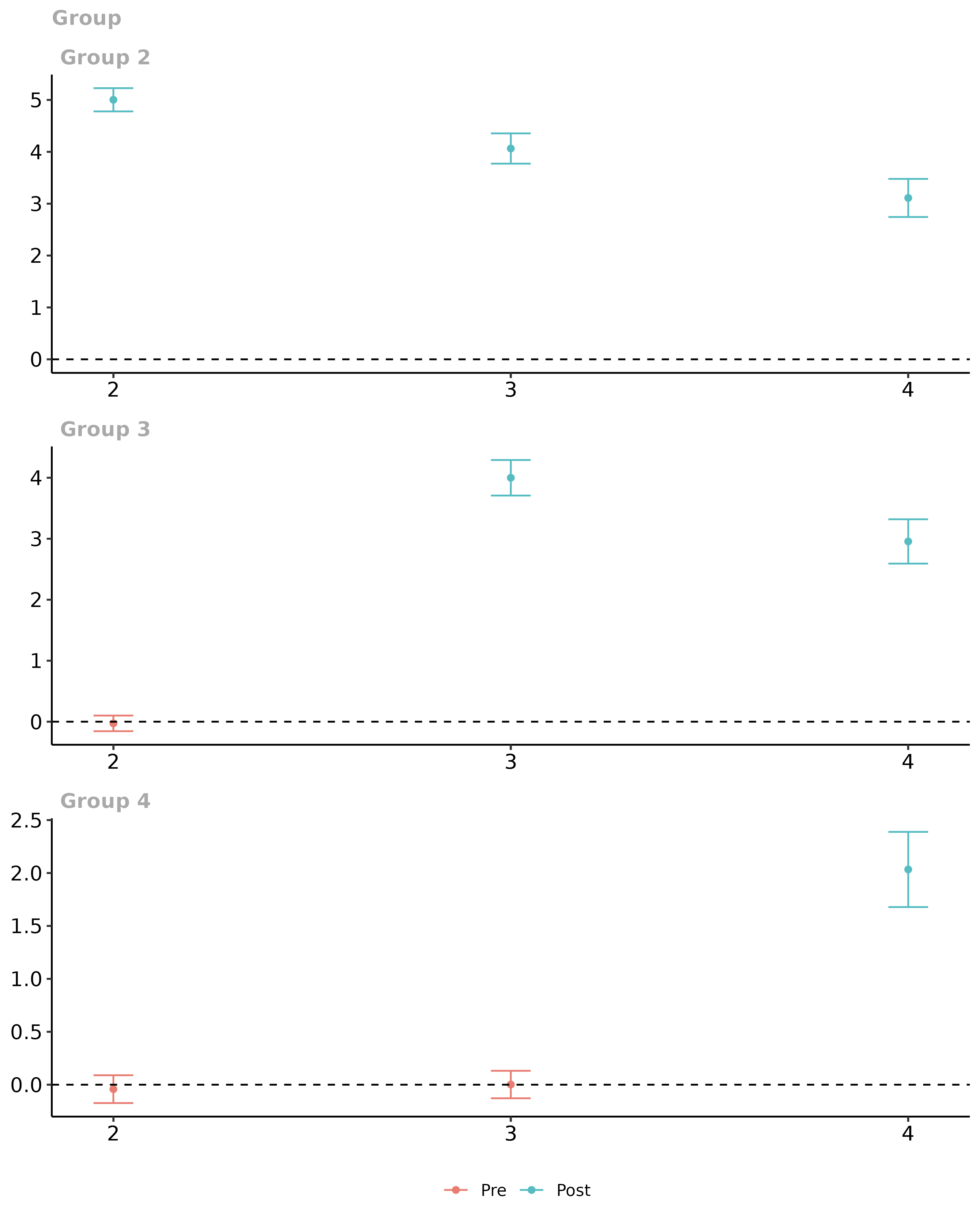
# aggregate them into event study plot
did.es <- aggte(did.att.gt, type = "dynamic")

# plot the event study
ggdid(did.es)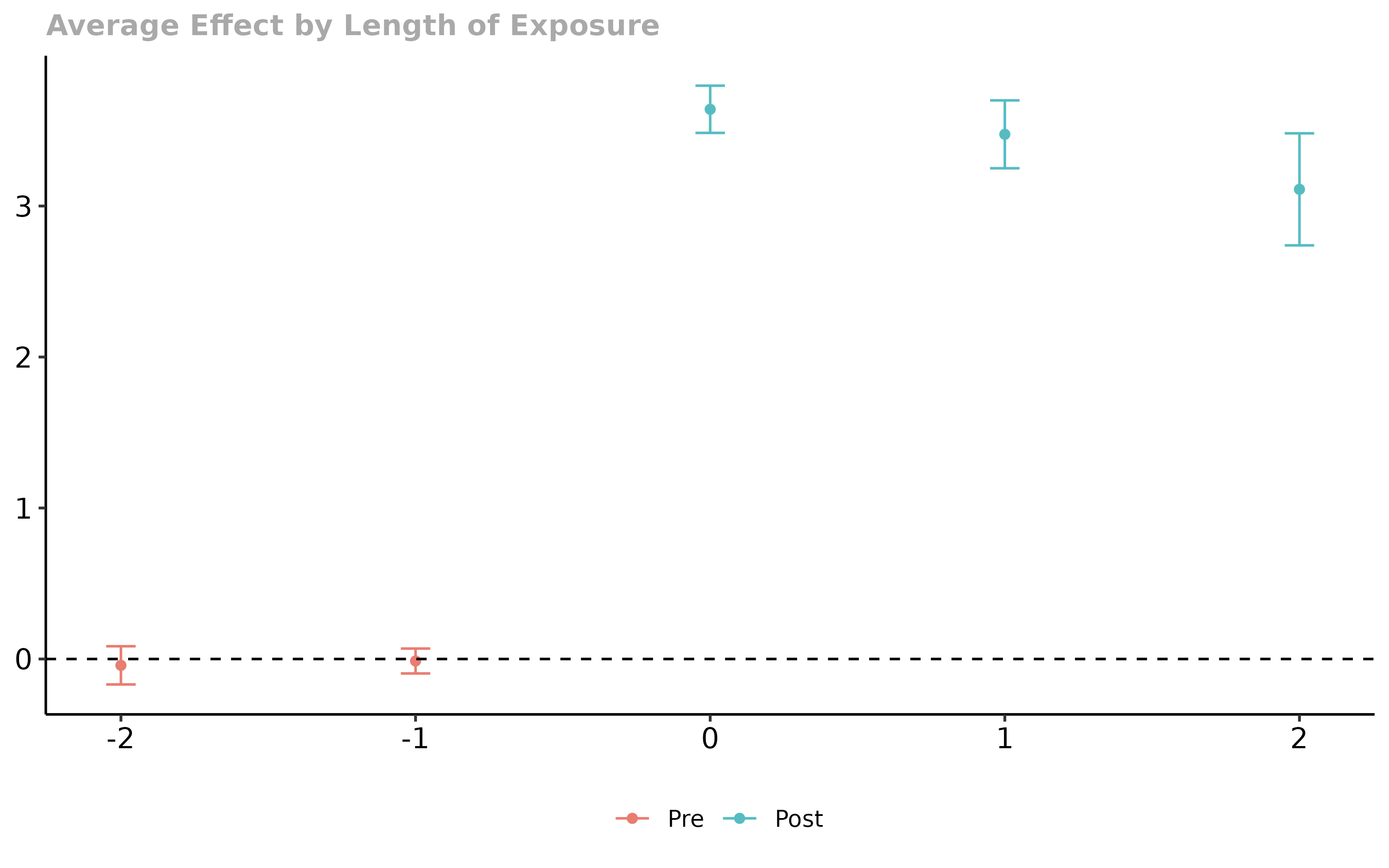
This is the correct performance (up to aforementioned caveats about multiple hypothesis testing).
Conditional Moment Tests
Another main use case for the did package is when the
parallel trends assumptions holds after conditioning on some covariates.
This is likely to be important in many applications. For example, to
evaluate the effect of participating in a job training program on
earnings, it is likely to be important to condition on an individual’s
education. This would be true if (i) the distribution of education is
different for individuals that participate in job training relative to
those that don’t (this is very likely to hold as people that participate
in job training tend to have less education than those who do not), and
(ii) if the path of earnings (absent participating in job training)
depends on an individual’s education. See Heckman, Ichimura, and Todd
(1998) and Abadie (2005) for more discussion.
Even when one includes covariates to estimate group-time average treatment effects, pre-tests based only on group-time average treatment effects can fail to detect some violations of the parallel trends assumption. To give an example, suppose that the only covariate is binary variable for an individual’s sex. Pre-tests based on group-time average treatment effects could fail to detect violations of the conditional parallel trends assumption in cases where it is violated in one direction for men and in the other direction for women.
The did package contains an additional pre-test for the
conditional parallel trends assumption in the
conditional_did_pretest function.
# not run (this code can be substantially slower)
reset.sim()
set.seed(1814)
nt <- 1000
nu <- 1000
cdp <- conditional_did_pretest("Y", "period", "id", "G", xformla = ~X, data = data)
cdp