unc_qte — unc_qte • qte

Estimates the Quantile Treatment Effect (QTE) or Quantile Treatment Effect on the Treated (QTT) under unconfoundedness, also known as selection on observables. The key identifying assumption is \((Y(0), Y(1)) \perp D \mid X\), i.e., potential outcomes are independent of treatment conditional on covariates \(X\).

Three estimation methods are available via est_method:

"ipw": Propensity-score reweighting (Firpo 2007). The propensity score \(p(X) = P(D=1|X)\) is estimated by logit or probit and used to reweight the sample so that the covariate distributions of the treated and untreated groups match. For the QTE, both groups are reweighted toward the population distribution; for the QTT, only the untreated group is reweighted toward the treated covariate distribution.
"or": Outcome regression via quantile regression inversion. rq is fit on a dense internal grid of \(\tau\) values, yielding a conditional quantile function \(Q_{Y|X,D=j}(\tau)\) for each arm \(j\). The marginal distribution is recovered by averaging conditional quantile functions over the empirical covariate distribution (Melly 2006; Chernozhukov, Fernandez-Val, and Melly 2013).
"aipw": Doubly-robust augmented IPW. Combines the propensity score model with the conditional quantile outcome model. The CDF estimator is consistent if either the propensity score or the outcome model is correctly specified (semiparametric efficiency when both are correct).

When xformla = ~1 (the default), all three methods reduce to simple quantile differences between the treated and untreated groups, which is consistent under unconditional unconfoundedness. Covariates are required for covariate-adjusted estimation.

Standard errors and uniform confidence bands are computed via the empirical bootstrap. Setting biters = 0 is planned for a future version to skip inference and return point estimates only.

Usage

unc_qte(
  yname,
  dname,
  data,
  xformla = ~1,
  weightsname = NULL,
  probs = seq(0.05, 0.95, 0.05),
  alp = 0.05,
  biters = 100,
  cband = TRUE,
  boot_type = "empirical",
  method = c("logit", "probit"),
  est_method = c("ipw", "or", "aipw"),
  target = c("qte", "qtt"),
  cl = 1
)

Arguments

yname

character; name of the outcome variable in data.

dname

character; name of the binary treatment indicator in data (1 = treated, 0 = untreated).

data

data.frame containing the analysis data.

xformla

one-sided formula for covariates used in the propensity score and/or outcome model, e.g. ~ age + I(age^2) + education. Default ~1 uses no covariates (simple quantile differences).

weightsname

character; name of a column in data containing sampling weights. Default NULL applies equal weights.

probs

numeric vector of quantile levels at which to evaluate the QTE or QTT. Default seq(0.05, 0.95, 0.05).

alp

significance level for confidence intervals. Default 0.05.

biters

number of bootstrap iterations for standard errors and confidence bands. Default 100.

cband

logical; if TRUE (default), report a uniform confidence band (simultaneous over all quantiles in probs) in addition to pointwise intervals.

boot_type

bootstrap variant. Currently only "empirical" is supported.

method

propensity score link function: "logit" (default) or "probit". Used by est_method = "ipw" and "aipw".

est_method

estimation method; one of:

"ipw" (default) — inverse propensity weighting
"or" — outcome regression via quantile regression inversion
"aipw" — doubly-robust augmented IPW

target

target parameter; one of:

"qte" (default) — population QTE: \(Q_{Y(1)}(\tau) - Q_{Y(0)}(\tau)\)
"qtt" — QTT (effect on the treated): \(Q_{Y(1)|D=1}(\tau) - Q_{Y(0)|D=1}(\tau)\)

cl

number of cores for parallel bootstrap. Default 1 (sequential).

Value

An object of class QTE containing:

qte: numeric vector of estimated QTE (or QTT) at each element of probs.
ate: estimated ATE (or ATT when target = "qtt").
qte.se: bootstrap standard errors for qte.
qte.lower, qte.upper: confidence interval bounds for qte; uniform when cband = TRUE, pointwise otherwise.
ate.se, ate.lower, ate.upper: SE and CI for ate.
probs: the probs vector passed by the user.
pscore.reg: fitted propensity score glm object, or NULL when est_method = "or" or xformla = ~1.

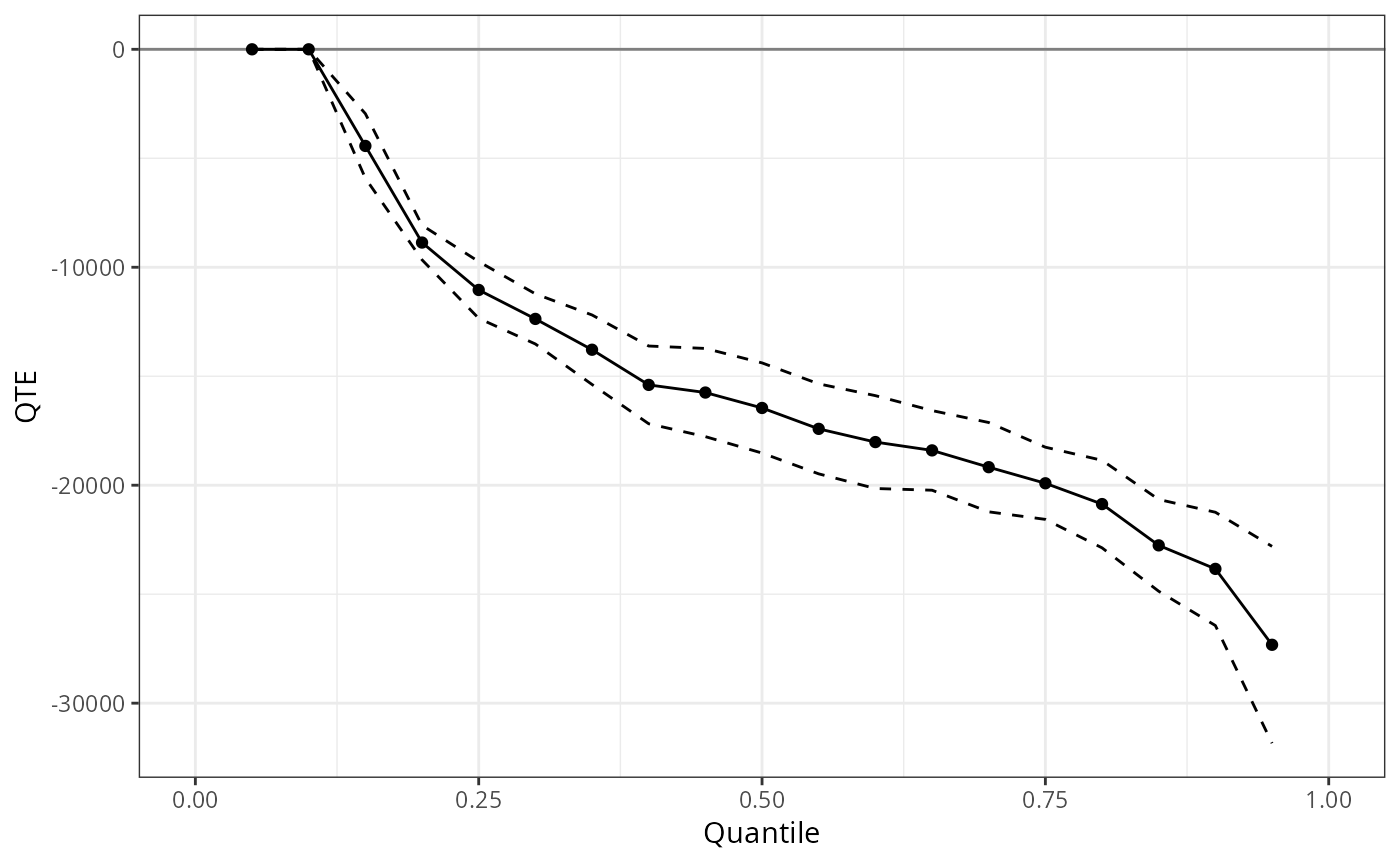
Use summary() to print a formatted table and plot() to display the QTE curve with confidence bands.

References

Firpo, Sergio. “Efficient Semiparametric Estimation of Quantile Treatment Effects.” Econometrica 75(1), pp. 259–276, 2007.

Melly, Blaise. “Estimation of Counterfactual Distributions Using Quantile Regression.” Working paper, University of St. Gallen, 2006.

Chernozhukov, Victor, Ivan Fernandez-Val, and Blaise Melly. “Inference on Counterfactual Distributions.” Econometrica 81(6), pp. 2205–2268, 2013.

Examples

data(lalonde)

## IPW, no covariates (simple quantile differences)
# \donttest{
q1 <- unc_qte(yname = "re78", dname = "treat", data = lalonde.psid,
              biters = 20, probs = seq(0.05, 0.95, 0.05))
summary(q1)
#> 
#> Overall ATE:  
#>        ATE    Std. Error     [ 95%  Conf. Int.]  
#>  -15204.78      658.7371  -16495.88   -13913.67 *
#> 
#> 
#> QTE:
#>   Tau        QTE Std. Error [ 95% Simult.  Conf. Band]  
#>  0.05      0.000     0.0000          0.000      0.0001 *
#>  0.10      0.000     0.0000          0.000      0.0000  
#>  0.15  -4433.180   755.5222      -5913.976  -2952.3833 *
#>  0.20  -8866.359   404.6120      -9659.384  -8073.3344 *
#>  0.25 -11041.037   664.4134     -12343.263  -9738.8102 *
#>  0.30 -12369.655   586.8586     -13519.877 -11219.4335 *
#>  0.35 -13783.867   813.5357     -15378.367 -12189.3659 *
#>  0.40 -15397.027   909.8757     -17180.351 -13613.7038 *
#>  0.45 -15747.885  1032.2459     -17771.050 -13724.7204 *
#>  0.50 -16455.862  1054.9852     -18523.595 -14388.1291 *
#>  0.55 -17414.162  1053.3812     -19478.751 -15349.5724 *
#>  0.60 -18020.487  1086.8987     -20150.769 -15890.2043 *
#>  0.65 -18402.105   932.1658     -20229.117 -16575.0939 *
#>  0.70 -19172.183  1045.4179     -21221.164 -17123.2013 *
#>  0.75 -19911.531   844.7875     -21567.285 -18255.7783 *
#>  0.80 -20865.535  1024.7453     -22873.999 -18857.0711 *
#>  0.85 -22759.664  1074.1332     -24864.927 -20654.4016 *
#>  0.90 -23838.991  1326.0996     -26438.098 -21239.8837 *
#>  0.95 -27321.670  2304.1312     -31837.684 -22805.6561 *
#> ---
#> Signif. codes: `*' confidence band does not cover 0
#> 
plot(q1)

# }

## OR with covariates, QTE
# \donttest{
xf <- ~ age + I(age^2) + education + black + hispanic + married + nodegree
q2 <- unc_qte(yname = "re78", dname = "treat", data = lalonde.psid,
              xformla = xf, est_method = "or",
              biters = 20, probs = seq(0.05, 0.95, 0.05))
summary(q2)
#> 
#> Overall ATE:  
#>     ATE    Std. Error     [ 95%  Conf. Int.]  
#>  -11673      1237.144  -14097.76   -9248.246 *
#> 
#> 
#> QTE:
#>   Tau         QTE Std. Error [ 95% Simult.  Conf. Band]  
#>  0.05      0.0000   534.0282      -1046.676   1046.6760  
#>  0.10   -629.4847   570.9274      -1748.482    489.5125  
#>  0.15  -3339.6661   792.9824      -4893.883  -1785.4493 *
#>  0.20  -6271.0174   983.1231      -8197.903  -4344.1314 *
#>  0.25  -7389.0936  1099.2800      -9543.643  -5234.5444 *
#>  0.30  -8720.8441  1011.3089     -10702.973  -6738.7151 *
#>  0.35  -9806.8096  1047.2833     -11859.447  -7754.1721 *
#>  0.40 -10691.4275  1252.9665     -13147.197  -8235.6584 *
#>  0.45 -11766.7929  1420.9047     -14551.715  -8981.8707 *
#>  0.50 -12340.5998  1521.6435     -15322.966  -9358.2334 *
#>  0.55 -13234.5395  1617.5103     -16404.801 -10064.2776 *
#>  0.60 -14019.6732  1696.7175     -17345.178 -10694.1681 *
#>  0.65 -14218.2984  1743.5961     -17635.684 -10800.9128 *
#>  0.70 -14998.7512  1923.6990     -18769.132 -11228.3705 *
#>  0.75 -15976.4066  2147.3183     -20185.073 -11767.7400 *
#>  0.80 -16608.3944  2399.6631     -21311.648 -11905.1412 *
#>  0.85 -18163.3251  2537.9927     -23137.699 -13188.9508 *
#>  0.90 -19352.5860  3017.5456     -25266.867 -13438.3053 *
#>  0.95 -21652.2255  4315.4411     -30110.335 -13194.1164 *
#> ---
#> Signif. codes: `*' confidence band does not cover 0
#> 
# }

## AIPW with covariates, QTT
# \donttest{
q3 <- unc_qte(yname = "re78", dname = "treat", data = lalonde.psid,
              xformla = xf, est_method = "aipw", target = "qtt",
              biters = 20, probs = seq(0.05, 0.95, 0.05))
summary(q3)
#> 
#> Overall ATT:  
#>        ATT    Std. Error     [ 95%  Conf. Int.]  
#>  -4685.583      1011.927  -6668.923   -2702.243 *
#> 
#> 
#> QTT:
#>   Tau         QTT Std. Error [ 95% Simult.  Conf. Band]  
#>  0.05      0.0001     0.0000         0.0001      0.0001 *
#>  0.10      0.0001     0.0000         0.0001      0.0001 *
#>  0.15      0.0001   383.8113      -752.2563    752.2564  
#>  0.20  -1002.7420   574.5027     -2128.7465    123.2625  
#>  0.25  -1866.2895  1081.3499     -3985.6964    253.1174  
#>  0.30  -3400.5673  1625.2306     -6585.9609   -215.1738 *
#>  0.35  -4425.4366  1709.7962     -7776.5756  -1074.2977 *
#>  0.40  -5009.2491  1332.0766     -7620.0712  -2398.4269 *
#>  0.45  -4673.7768  1296.9578     -7215.7674  -2131.7861 *
#>  0.50  -4602.4652  1117.7569     -6793.2285  -2411.7020 *
#>  0.55  -4579.3967  1169.9553     -6872.4670  -2286.3264 *
#>  0.60  -5229.1685  1257.1331     -7693.1040  -2765.2330 *
#>  0.65  -5101.4965  1256.5516     -7564.2924  -2638.7006 *
#>  0.70  -5507.4720  1177.2351     -7814.8104  -3200.1336 *
#>  0.75  -6367.7241  1303.4433     -8922.4260  -3813.0223 *
#>  0.80  -6885.7529  1502.1072     -9829.8289  -3941.6769 *
#>  0.85  -8075.3068  1816.4340    -11635.4520  -4515.1617 *
#>  0.90 -10517.0625  2167.8397    -14765.9502  -6268.1749 *
#>  0.95 -10757.3772  2919.2854    -16479.0715  -5035.6829 *
#> ---
#> Signif. codes: `*' confidence band does not cover 0
#> 
# }