load("job_displacement_data.RData")Exercise 1 Solutions
This exercise will involve estimating causal effect parameters using a difference-in-differences identification strategy that involves conditioning on covariates in the parallel trends assumption and possibly allows for anticipation effects.
In particular, we will use data from the National Longitudinal Study of Youth to learn about causal effects of job displacement (where job displacement roughly means “losing your job through no fault of your own” — a mass layoff is a main example).
To start with, load the data from the file job_displacement_data.RData by running
which will load a data.frame called job_displacement_data. This is what the data looks like
head(job_displacement_data) id year group income female white occ_score
1 7900002 1984 0 31130 1 1 4
2 7900002 1985 0 32200 1 1 3
3 7900002 1986 0 35520 1 1 4
4 7900002 1987 0 43600 1 1 4
5 7900002 1988 0 39900 1 1 4
6 7900002 1990 0 38200 1 1 4You can see that the data contains the following columns:
id- an individual identifieryear- the year for this observationgroup- the year that person lost his/her job.group=0for those that do not lose a job in any period being considered.income- a person’s wage and salary income in this yearfemale- 1 for females, 0 for maleswhite- 1 for white, 0 for non-white
For the results below, we will mainly use the did package which you can install using install.packages("did"), and you can load it using
library(did)Question 1
We will start by computing group-time average treatment effects without including any covariates in the parallel trends assumption.
- Use the
didpackage to compute all available group-time average treatment effects.
Solutions:
no_covs <- att_gt(yname="income",
                  tname="year",
                  idname="id",
                  gname="group",
                  data=job_displacement_data)
Warning in pre_process_did(yname = yname, tname = tname, idname = idname, :
Dropped 26 units that were already treated in the first period.summary(no_covs)
Call:
att_gt(yname = "income", tname = "year", idname = "id", gname = "group",
    data = job_displacement_data)

Reference: Callaway, Brantly and Pedro H.C. Sant'Anna.  "Difference-in-Differences with Multiple Time Periods." Journal of Econometrics, Vol. 225, No. 2, pp. 200-230, 2021. <https://doi.org/10.1016/j.jeconom.2020.12.001>, <https://arxiv.org/abs/1803.09015>

Group-Time Average Treatment Effects:
 Group Time    ATT(g,t) Std. Error [95% Simult.  Conf. Band]
  1985 1985  -9455.7583   3861.042   -19528.8115    617.2948
  1985 1986 -14981.1547   4673.005   -27172.5348  -2789.7746 *
  1985 1987  -6129.2132   4200.985   -17089.1417   4830.7153
  1985 1988  -4815.9179   4980.184   -17808.6958   8176.8600
  1985 1990  -8011.9173   5466.432   -22273.2656   6249.4310
  1985 1991  -8164.4924   6444.642   -24977.8874   8648.9026
  1985 1992  -6325.8880   5779.045   -21402.8090   8751.0330
  1985 1993  -9669.5840   5527.646   -24090.6329   4751.4649
  1986 1985  -1801.9373   2599.738    -8584.3796   4980.5051
  1986 1986  -1919.4474   3510.325   -11077.5154   7238.6207
  1986 1987  -2596.8189   4846.428   -15240.6413  10047.0034
  1986 1988  -2081.7535   6986.801   -20309.5851  16146.0782
  1986 1990  -6064.0942   6633.956   -23371.3876  11243.1992
  1986 1991  -5903.9636   6766.574   -23557.2437  11749.3164
  1986 1992  -6804.4833   7425.492   -26176.8110  12567.8445
  1986 1993  -1801.5755   7455.891   -21253.2138  17650.0628
  1987 1985   4518.5745   5248.997    -9175.5067  18212.6557
  1987 1986  -8012.4879   4547.337   -19876.0119   3851.0360
  1987 1987   7048.8565   6692.480   -10411.1225  24508.8355
  1987 1988   4489.4666   6807.248   -13269.9275  22248.8608
  1987 1990   8004.1361   6737.479    -9573.2386  25581.5108
  1987 1991   9475.0656   7284.194    -9528.6318  28478.7630
  1987 1992   8533.5413  10080.963   -17766.6333  34833.7160
  1987 1993   7881.3931   7330.973   -11244.3452  27007.1314
  1988 1985  -8350.7706   4631.991   -20435.1498   3733.6085
  1988 1986  -3420.8529   3637.104   -12909.6754   6067.9695
  1988 1987  -3617.6742   3493.304   -12731.3380   5495.9897
  1988 1988  -1173.8167   3174.614    -9456.0523   7108.4190
  1988 1990    280.6263   5825.393   -14917.2132  15478.4658
  1988 1991   6099.7271   4046.620    -4457.4799  16656.9341
  1988 1992  13737.8166  12846.521   -19777.4078  47253.0410
  1988 1993   1688.7819   8220.831   -19758.5022  23136.0659
  1990 1985  -5281.5363   3433.800   -14239.9612   3676.8886
  1990 1986   3654.1728   2560.200    -3025.1209  10333.4664
  1990 1987   5934.8952   3040.891    -1998.4696  13868.2599
  1990 1988   1034.1988   3161.435    -7213.6530   9282.0505
  1990 1990  -4343.9488  12267.489   -36348.5390  27660.6414
  1990 1991 -21910.2102   4908.635   -34716.3237  -9104.0966 *
  1990 1992 -15365.9271   3994.383   -25786.8532  -4945.0010 *
  1990 1993 -16411.1053   6244.878   -32703.3363   -118.8743 *
  1991 1985    891.2874   3590.076    -8474.8439  10257.4186
  1991 1986  -2816.6357   3576.210   -12146.5924   6513.3211
  1991 1987  -1340.0549   3135.896    -9521.2781   6841.1683
  1991 1988  -7025.0387   3718.362   -16725.8557   2675.7782
  1991 1990   2568.6223   6028.719   -13159.6720  18296.9167
  1991 1991 -12150.6450   4287.933   -23337.4115   -963.8784 *
  1991 1992   1433.9979   4595.143   -10554.2472  13422.2430
  1991 1993  -2679.8275   7112.789   -21236.3485  15876.6935
  1992 1985 -12110.0572   6180.931   -28235.4586   4015.3442
  1992 1986  -3287.5606   2537.390    -9907.3443   3332.2230
  1992 1987   2300.0285   3528.032    -6904.2362  11504.2931
  1992 1988  -7273.9345   2714.144   -14354.8502   -193.0189 *
  1992 1990   7351.4926   4801.529    -5175.1936  19878.1788
  1992 1991 -10031.7028   7619.266   -29909.5691   9846.1636
  1992 1992  -8990.8504   4258.882   -20101.8273   2120.1264
  1992 1993  -8662.6119  14973.627   -47727.2335  30402.0097
  1993 1985  -7424.6641   5468.588   -21691.6364   6842.3081
  1993 1986    677.9060   3381.472    -8143.9982   9499.8102
  1993 1987   1424.1385   3835.053    -8581.1117  11429.3886
  1993 1988   4778.2556   1746.084      222.9054   9333.6057 *
  1993 1990  -3797.3928   4628.671   -15873.1102   8278.3246
  1993 1991   3664.8825   6840.202   -14180.4872  21510.2523
  1993 1992  -4108.9169   5801.940   -19245.5705  11027.7368
  1993 1993 -22828.3617   6567.402   -39962.0233  -5694.7001 *
---
Signif. codes: `*' confidence band does not cover 0

P-value for pre-test of parallel trends assumption:  0
Control Group:  Never Treated,  Anticipation Periods:  0
Estimation Method: Doubly Robust- Bonus Question Try to manually calculate \(ATT(g=1992, t=1992)\). Can you calculate exactly the same number as in part (a)?
Solutions:
  mean(subset(job_displacement_data, group==1992 & year==1992)$income) -
    mean(subset(job_displacement_data, group==1992 & year==1991)$income) -
    ( mean(subset(job_displacement_data, group==0 & year==1992)$income) -
    mean(subset(job_displacement_data, group==0 & year==1991)$income) )
[1] -8990.85- Aggregate the group-time average treatment effects into an event study and plot the results. What do you notice? Is there evidence against parallel trends?
Solutions:
  no_covs_es <- aggte(no_covs, type="dynamic")
  ggdid(no_covs_es)
- Aggregate the group-time average treatment effects into a single overall treatment effect. How do you interpret the results?
Solutions:
  no_covs_overall <- aggte(no_covs, type="group")
  summary(no_covs_overall)
Call:
aggte(MP = no_covs, type = "group")

Reference: Callaway, Brantly and Pedro H.C. Sant'Anna.  "Difference-in-Differences with Multiple Time Periods." Journal of Econometrics, Vol. 225, No. 2, pp. 200-230, 2021. <https://doi.org/10.1016/j.jeconom.2020.12.001>, <https://arxiv.org/abs/1803.09015>


Overall summary of ATT's based on group/cohort aggregation:
       ATT    Std. Error     [ 95%  Conf. Int.]
 -5631.049      2009.565  -9569.723   -1692.374 *


Group Effects:
 Group   Estimate Std. Error [95% Simult.  Conf. Band]
  1985  -8444.241   4700.126    -19889.596    3001.115
  1986  -3881.734   6126.311    -18800.018   11036.550
  1987   7572.077   6619.391     -8546.914   23691.067
  1988   4126.627   4890.516     -7782.349   16035.603
  1990 -14507.798   4355.249    -25113.338   -3902.258 *
  1991  -4465.492   4715.478    -15948.230    7017.247
  1992  -8826.731   8360.343    -29185.143   11531.681
  1993 -22828.362   6462.085    -38564.294   -7092.429 *
---
Signif. codes: `*' confidence band does not cover 0

Control Group:  Never Treated,  Anticipation Periods:  0
Estimation Method:  Doubly Robust
Question 2
A major issue in the job displacement literature concerns a version of anticipation. In particular, there is some empirical evidence that earnings of displaced workers start to decline before they are actually displaced (a rough explanation is that firms where there are mass layoffs typically “struggle” in the time period before the mass layoff actually takes place and this can lead to slower income growth for workers at those firms).
- Is there evidence of anticipation in your results from Question 1?
Solutions:
There is a moderate amount of evidence for anticipation in the previous results. It hinges on the estimate for event-time equal to -1. It is negative which is in line with the discussion about anticipation above, but it is only marginally statistically significant.
- Repeat parts (a)-(d) of Question 1 allowing for one year of anticipation.
Solutions:
  # part a
  ant_res <- att_gt(yname="income",
                    tname="year",
                    idname="id",
                    gname="group",
                    data=job_displacement_data,
                    anticipation=1)
Warning in pre_process_did(yname = yname, tname = tname, idname = idname, :
Dropped 26 units that were already treated in the first period. summary(ant_res)
Call:
att_gt(yname = "income", tname = "year", idname = "id", gname = "group",
    data = job_displacement_data, anticipation = 1)

Reference: Callaway, Brantly and Pedro H.C. Sant'Anna.  "Difference-in-Differences with Multiple Time Periods." Journal of Econometrics, Vol. 225, No. 2, pp. 200-230, 2021. <https://doi.org/10.1016/j.jeconom.2020.12.001>, <https://arxiv.org/abs/1803.09015>

Group-Time Average Treatment Effects:
 Group Time    ATT(g,t) Std. Error [95% Simult.  Conf. Band]
  1986 1985  -1801.9373   2637.305    -8447.6078   4843.7333
  1986 1986  -3721.3846   3692.454   -13025.8967   5583.1275
  1986 1987  -4398.7562   4035.808   -14568.4747   5770.9624
  1986 1988  -3883.6907   6377.636   -19954.5162  12187.1347
  1986 1990  -7866.0314   6149.536   -23362.0739   7630.0110
  1986 1991  -7705.9009   6433.556   -23917.6395   8505.8378
  1986 1992  -8606.4205   6922.425   -26050.0443   8837.2032
  1986 1993  -3603.5128   6755.388   -20626.2250  13419.1995
  1987 1985   4518.5745   5460.994    -9242.4313  18279.5803
  1987 1986  -8012.4879   4701.940   -19860.7751   3835.7992
  1987 1987   -963.6314   7276.588   -19299.7028  17372.4399
  1987 1988  -3523.0213   7994.976   -23669.3383  16623.2957
  1987 1990     -8.3518   6296.508   -15874.7459  15858.0423
  1987 1991   1462.5776   7589.264   -17661.3964  20586.5516
  1987 1992    521.0534   9526.404   -23484.2640  24526.3708
  1987 1993   -131.0948   7403.803   -18787.7296  18525.5399
  1988 1985  -8350.7706   4674.623   -20130.2233   3428.6820
  1988 1986  -3420.8529   3463.723   -12148.9916   5307.2858
  1988 1987  -3617.6742   3619.131   -12737.4217   5502.0734
  1988 1988  -4791.4908   4401.680   -15883.1619   6300.1802
  1988 1990  -3337.0478   8180.250   -23950.2306  17276.1349
  1988 1991   2482.0529   6363.899   -13554.1573  18518.2632
  1988 1992  10120.1424  14533.152   -26501.5387  46741.8236
  1988 1993  -1928.8923   7476.284   -20768.1705  16910.3860
  1990 1985  -5281.5363   3373.666   -13782.7425   3219.6699
  1990 1986   3654.1728   2480.289    -2595.8377   9904.1833
  1990 1987   5934.8952   2890.621    -1349.0994  13218.8897
  1990 1988   1034.1988   3167.434    -6947.3291   9015.7266
  1990 1990  -4343.9488  12209.279   -35109.7687  26421.8712
  1990 1991 -21910.2102   4491.669   -33228.6418 -10591.7785 *
  1990 1992 -15365.9271   3899.003   -25190.9152  -5540.9391 *
  1990 1993 -16411.1053   6250.408   -32161.3325   -660.8781 *
  1991 1985    891.2874   3471.665    -7856.8633   9639.4380
  1991 1986  -2816.6357   3552.765   -11769.1484   6135.8771
  1991 1987  -1340.0549   3332.791    -9738.2616   7058.1518
  1991 1988  -7025.0387   3873.773   -16786.4497   2736.3723
  1991 1990   2568.6223   6363.298   -13466.0749  18603.3196
  1991 1991  -9582.0227   9188.794   -32736.6064  13572.5611
  1991 1992   4002.6202   8634.215   -17754.4959  25759.7363
  1991 1993   -111.2052  10465.683   -26483.3858  26260.9755
  1992 1985 -12110.0572   6789.117   -29217.7628   4997.6484
  1992 1986  -3287.5606   2445.489    -9449.8803   2874.7591
  1992 1987   2300.0285   3451.590    -6397.5352  10997.5921
  1992 1988  -7273.9345   2662.708   -13983.6169   -564.2522 *
  1992 1990   7351.4926   4587.882    -4209.3820  18912.3673
  1992 1991 -10031.7028   7928.273   -30009.9359   9946.5304
  1992 1992 -19022.5532   7204.014   -37175.7451   -869.3614 *
  1992 1993 -18694.3146   8280.700   -39560.6188   2171.9895
  1993 1985  -7424.6641   5005.794   -20038.6230   5189.2947
  1993 1986    677.9060   3139.230    -7232.5509   8588.3629
  1993 1987   1424.1385   3873.730    -8337.1656  11185.4425
  1993 1988   4778.2556   1600.827      744.3767   8812.1344 *
  1993 1990  -3797.3928   4115.722   -14168.4854   6573.6998
  1993 1991   3664.8825   6713.530   -13252.3528  20582.1179
  1993 1992  -4108.9169   5524.881   -18030.9090   9813.0753
  1993 1993 -26937.2785   5418.226   -40590.5140 -13284.0431 *
---
Signif. codes: `*' confidence band does not cover 0

P-value for pre-test of parallel trends assumption:  0
Control Group:  Never Treated,  Anticipation Periods:  1
Estimation Method:  Doubly Robust
# part b
mean(subset(job_displacement_data, group==1992 & year==1992)$income) -
mean(subset(job_displacement_data, group==1992 & year==1990)$income) -
( mean(subset(job_displacement_data, group==0 & year==1992)$income) -
mean(subset(job_displacement_data, group==0 & year==1990)$income) )[1] -19022.55 # part c
ant_es <- aggte(ant_res, type="dynamic")
ggdid(ant_es)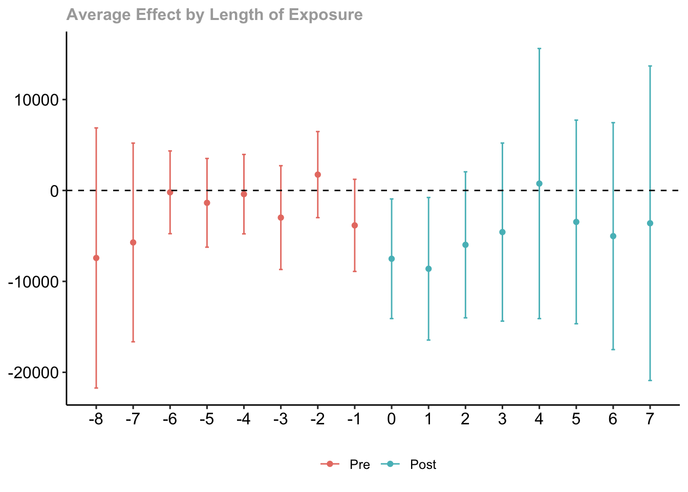
  # part d
  ant_overall <- aggte(ant_res, type="group")
  summary(ant_overall)
Call:
aggte(MP = ant_res, type = "group")

Reference: Callaway, Brantly and Pedro H.C. Sant'Anna.  "Difference-in-Differences with Multiple Time Periods." Journal of Econometrics, Vol. 225, No. 2, pp. 200-230, 2021. <https://doi.org/10.1016/j.jeconom.2020.12.001>, <https://arxiv.org/abs/1803.09015>


Overall summary of ATT's based on group/cohort aggregation:
       ATT    Std. Error     [ 95%  Conf. Int.]
 -7711.634      2327.567  -12273.58   -3149.686 *


Group Effects:
 Group    Estimate Std. Error [95% Simult.  Conf. Band]
  1986  -5683.6710   5470.628     -17794.15    6426.809
  1987   -440.4114   6497.956     -14825.12   13944.294
  1988    508.9529   6006.259     -12787.27   13805.175
  1990 -14507.7979   4197.887     -23800.78   -5214.819 *
  1991  -1896.8692   8323.324     -20322.44   16528.702
  1992 -18858.4339   4474.770     -28764.36   -8952.513 *
  1993 -26937.2785   5812.733     -39805.09  -14069.471 *
---
Signif. codes: `*' confidence band does not cover 0

Control Group:  Never Treated,  Anticipation Periods:  1
Estimation Method:  Doubly Robust
Question 3
Now, let’s suppose that we think that parallel trends holds only after we condition on a person sex and race (in reality, you could think of including many other variables in the parallel trends assumption, but let’s just keep it simple). In my view, I think allowing for anticipation is desirable in this setting too, so let’s keep allowing for one year of anticipation.
- Answer parts (a), (c), and (d) of Question 1 but including
sexandwhiteas covariates.
Solutions:
  # part a
  covs_res <- att_gt(yname="income",
                    tname="year",
                    idname="id",
                    gname="group",
                    data=job_displacement_data,
                    anticipation=1,
                    xformla=~female + white)
Warning in pre_process_did(yname = yname, tname = tname, idname = idname, :
Dropped 26 units that were already treated in the first period.Warning in pre_process_did(yname = yname, tname = tname, idname = idname, : Be aware that there are some small groups in your dataset.
Check groups: 1992,1993. summary(covs_res)
Call:
att_gt(yname = "income", tname = "year", idname = "id", gname = "group",
xformla = ~female + white, data = job_displacement_data,
anticipation = 1)
Reference: Callaway, Brantly and Pedro H.C. Sant'Anna. "Difference-in-Differences with Multiple Time Periods." Journal of Econometrics, Vol. 225, No. 2, pp. 200-230, 2021. <https://doi.org/10.1016/j.jeconom.2020.12.001>, <https://arxiv.org/abs/1803.09015>
Group-Time Average Treatment Effects:
Group Time ATT(g,t) Std. Error [95% Simult. Conf. Band]
1986 1985 -1724.0034 2493.960 -7957.3577 4509.3509
1986 1986 -4258.8672 3475.987 -12946.6795 4428.9451
1986 1987 -4861.6136 3901.328 -14612.5144 4889.2873
1986 1988 -4729.6121 6550.950 -21102.9257 11643.7016
1986 1990 -8685.9902 5919.644 -23481.4317 6109.4514
1986 1991 -8753.8554 6140.301 -24100.8026 6593.0917
1986 1992 -9530.3951 6819.824 -26575.7285 7514.9382
1986 1993 -4727.7652 6608.974 -21246.1040 11790.5736
1987 1985 4559.7049 5401.196 -8939.9374 18059.3472
1987 1986 -8337.6804 4628.947 -19907.1778 3231.8171
1987 1987 -1244.4854 7055.388 -18878.5822 16389.6114
1987 1988 -4009.1142 7547.463 -22873.0934 14854.8651
1987 1990 -483.2506 6510.734 -16756.0494 15789.5483
1987 1991 865.8558 7991.793 -19108.6731 20840.3847
1987 1992 -1.1369 9485.687 -23709.4748 23707.2010
1987 1993 -760.5834 7646.473 -19872.0265 18350.8596
1988 1985 -8427.9592 4483.846 -19634.7939 2778.8755
1988 1986 -3208.6634 3785.889 -12671.0400 6253.7133
1988 1987 -3540.3348 3667.076 -12705.7526 5625.0830
1988 1988 -4496.7178 4488.311 -15714.7134 6721.2778
1988 1990 -2886.2705 7805.516 -22395.2224 16622.6814
1988 1991 3026.1289 6141.168 -12322.9835 18375.2413
1988 1992 10422.7498 15019.310 -27116.2158 47961.7153
1988 1993 -1710.3233 7388.194 -20176.2295 16755.5830
1990 1985 -5423.4224 3557.666 -14315.3831 3468.5383
1990 1986 4124.3571 2819.216 -2921.9351 11170.6493
1990 1987 6034.5096 3012.839 -1495.7213 13564.7406
1990 1988 1473.8450 3277.915 -6718.9116 9666.6016
1990 1990 -4087.0904 12272.756 -34761.3721 26587.1913
1990 1991 -21451.7077 4889.978 -33673.6224 -9229.7929 *
1990 1992 -15350.4684 3736.307 -24688.9203 -6012.0165 *
1990 1993 -16489.8656 6266.352 -32151.8605 -827.8708 *
1991 1985 787.4357 3522.377 -8016.3237 9591.1950
1991 1986 -2463.7125 3696.944 -11703.7810 6776.3560
1991 1987 -1271.9440 3335.578 -9608.8221 7064.9341
1991 1988 -6698.7830 3813.606 -16230.4339 2832.8679
1991 1990 2753.4298 6037.666 -12336.9920 17843.8516
1991 1991 -9246.2829 8636.010 -30830.9534 12338.3877
1991 1992 4013.8999 8088.141 -16201.4400 24229.2398
1991 1993 -162.2495 10086.002 -25371.0029 25046.5038
1992 1985 -12170.1207 6394.614 -28152.6913 3812.4499
1992 1986 -3584.4939 2410.058 -9608.1443 2439.1566
1992 1987 2598.5246 3653.567 -6533.1284 11730.1775
1992 1988 -7330.9148 2871.569 -14508.0580 -153.7715 *
1992 1990 7649.2124 4740.277 -4198.5416 19496.9663
1992 1991 -10130.9141 7932.263 -29956.6541 9694.8259
1992 1992 -19327.7970 6701.003 -36076.1514 -2579.4426 *
1992 1993 -19410.4421 8689.023 -41127.6126 2306.7284
1993 1985 -7391.9287 5580.167 -21338.8875 6555.0302
1993 1986 50.7636 3523.194 -8755.0376 8856.5648
1993 1987 1618.3041 3763.007 -7786.8800 11023.4883
1993 1988 4453.4544 1769.420 31.0011 8875.9077 *
1993 1990 -3630.4984 3887.086 -13345.8049 6084.8080
1993 1991 3439.7874 6512.448 -12837.2945 19716.8692
1993 1992 -4123.7577 5953.866 -19004.7314 10757.2161
1993 1993 -27304.4090 5711.372 -41579.2990 -13029.5190 *
---
Signif. codes: `*' confidence band does not cover 0
P-value for pre-test of parallel trends assumption: 0
Control Group: Never Treated, Anticipation Periods: 1
Estimation Method: Doubly Robust # part c
covs_es <- aggte(covs_res, type="dynamic")
ggdid(covs_es)
# part d
covs_overall <- aggte(covs_res, type="group")
summary(covs_overall)
Call:
aggte(MP = covs_res, type = "group")
Reference: Callaway, Brantly and Pedro H.C. Sant'Anna. "Difference-in-Differences with Multiple Time Periods." Journal of Econometrics, Vol. 225, No. 2, pp. 200-230, 2021. <https://doi.org/10.1016/j.jeconom.2020.12.001>, <https://arxiv.org/abs/1803.09015>
Overall summary of ATT's based on group/cohort aggregation:
ATT Std. Error [ 95% Conf. Int.]
-7931.965 2389.043 -12614.4 -3249.526 *
Group Effects:
Group Estimate Std. Error [95% Simult. Conf. Band]
1986 -6506.8712 5271.801 -18120.53 5106.783
1987 -938.7858 6869.413 -16071.94 14194.369
1988 871.1134 6286.149 -12977.12 14719.352
1990 -14344.7830 4317.628 -23856.42 -4833.149 *
1991 -1798.2108 8271.638 -20020.44 16424.014
1992 -19369.1196 4406.584 -29076.72 -9661.517 *
1993 -27304.4090 5819.843 -40125.39 -14483.431 *
---
Signif. codes: `*' confidence band does not cover 0
Control Group: Never Treated, Anticipation Periods: 1
Estimation Method: Doubly Robust- By default, the
didpackage uses the doubly robust approach that we discussed during our session. How do the results change if you use a regression approach or propensity score re-weighting?
Solutions:
For simplicity, I am just going to show the overall results when using the regression approach and the propensity score re-weighting approach.
reg_res <- att_gt(yname="income",
tname="year",
idname="id",
gname="group",
data=job_displacement_data,
anticipation=1,
xformla=~female + white,
est_method="reg")Warning in pre_process_did(yname = yname, tname = tname, idname = idname, :
Dropped 26 units that were already treated in the first period.Warning in pre_process_did(yname = yname, tname = tname, idname = idname, : Be aware that there are some small groups in your dataset.
Check groups: 1992,1993. summary(aggte(reg_res, type="group"))
Call:
aggte(MP = reg_res, type = "group")
Reference: Callaway, Brantly and Pedro H.C. Sant'Anna. "Difference-in-Differences with Multiple Time Periods." Journal of Econometrics, Vol. 225, No. 2, pp. 200-230, 2021. <https://doi.org/10.1016/j.jeconom.2020.12.001>, <https://arxiv.org/abs/1803.09015>
Overall summary of ATT's based on group/cohort aggregation:
ATT Std. Error [ 95% Conf. Int.]
-7919.691 2241.563 -12313.07 -3526.308 *
Group Effects:
Group Estimate Std. Error [95% Simult. Conf. Band]
1986 -6434.0559 5552.204 -18399.92 5531.812
1987 -912.7508 6601.460 -15139.93 13314.428
1988 862.1890 6513.785 -13176.04 14900.415
1990 -14343.8838 4120.677 -23224.59 -5463.180 *
1991 -1796.2167 8395.139 -19889.05 16296.621
1992 -19441.0738 4325.936 -28764.14 -10118.005 *
1993 -27302.1029 5815.805 -39836.07 -14768.134 *
---
Signif. codes: `*' confidence band does not cover 0
Control Group: Never Treated, Anticipation Periods: 1
Estimation Method: Outcome Regression ipw_res <- att_gt(yname="income",
tname="year",
idname="id",
gname="group",
data=job_displacement_data,
anticipation=1,
xformla=~female + white,
est_method="ipw")Warning in pre_process_did(yname = yname, tname = tname, idname = idname, : Dropped 26 units that were already treated in the first period.
Warning in pre_process_did(yname = yname, tname = tname, idname = idname, : Be aware that there are some small groups in your dataset.
Check groups: 1992,1993. summary(aggte(ipw_res, type="group"))
Call:
aggte(MP = ipw_res, type = "group")

Reference: Callaway, Brantly and Pedro H.C. Sant'Anna.  "Difference-in-Differences with Multiple Time Periods." Journal of Econometrics, Vol. 225, No. 2, pp. 200-230, 2021. <https://doi.org/10.1016/j.jeconom.2020.12.001>, <https://arxiv.org/abs/1803.09015>


Overall summary of ATT's based on group/cohort aggregation:
      ATT    Std. Error     [ 95%  Conf. Int.]
 -7931.69      2395.857  -12627.48   -3235.896 *


Group Effects:
 Group    Estimate Std. Error [95% Simult.  Conf. Band]
  1986  -6506.2796   5366.182     -18329.69    5317.130
  1987   -938.6980   7027.544     -16422.62   14545.222
  1988    871.1522   5952.535     -12244.18   13986.484
  1990 -14345.0498   4649.411     -24589.19   -4100.914 *
  1991  -1798.1771   8179.503     -19820.23   16223.875
  1992 -19368.1395   4545.188     -29382.64   -9353.642 *
  1993 -27303.3746   5786.646     -40053.20  -14553.548 *
---
Signif. codes: `*' confidence band does not cover 0

Control Group:  Never Treated,  Anticipation Periods:  1
Estimation Method:  Inverse Probability Weighting
You can see that the results are very similar across estimation strategies in this example.
Question 4
Finally, the data that we have contains a variable called occ_score which is roughly a variable that measures the occupation “quality”. Suppose that we (i) are interested in including a person’s occupation in the parallel trends assumption, (ii) are satisfied that occ_score sufficiently summarizes a person’s occupation, but (iii) are worried that a person’s occupation is a “bad control” (in the sense that it could be affected by the treatment).
- Repeat parts (a), (c), and (d) of Question 1 but including
occ_scorein the parallel trends assumption. Continue to allow for 1 year of anticipation effects.
Solutions:
  # part a
  occ_res <- att_gt(yname="income",
                    tname="year",
                    idname="id",
                    gname="group",
                    data=job_displacement_data,
                    anticipation=1,
                    xformla=~female + white + occ_score)
Warning in pre_process_did(yname = yname, tname = tname, idname = idname, :
Dropped 26 units that were already treated in the first period.Warning in pre_process_did(yname = yname, tname = tname, idname = idname, : Be aware that there are some small groups in your dataset.
Check groups: 1992,1993. summary(occ_res)
Call:
att_gt(yname = "income", tname = "year", idname = "id", gname = "group",
    xformla = ~female + white + occ_score, data = job_displacement_data,
    anticipation = 1)

Reference: Callaway, Brantly and Pedro H.C. Sant'Anna.  "Difference-in-Differences with Multiple Time Periods." Journal of Econometrics, Vol. 225, No. 2, pp. 200-230, 2021. <https://doi.org/10.1016/j.jeconom.2020.12.001>, <https://arxiv.org/abs/1803.09015>

Group-Time Average Treatment Effects:
 Group Time    ATT(g,t) Std. Error [95% Simult.  Conf. Band]
  1986 1985  -2195.2252   2439.588     -8404.432   4013.9820
  1986 1986  -4943.5726   3602.994    -14113.864   4226.7192
  1986 1987  -5648.5248   4289.363    -16565.754   5268.7046
  1986 1988  -5486.8776   6630.855    -22363.640  11389.8853
  1986 1990  -9355.8673   5982.470    -24582.370   5870.6353
  1986 1991  -9341.8431   6334.782    -25465.046   6781.3597
  1986 1992 -10108.9739   6896.816    -27662.657   7444.7096
  1986 1993  -5529.8989   6878.792    -23037.708  11977.9101
  1987 1985   3820.8904   5398.740     -9919.911  17561.6916
  1987 1986  -8340.0613   4527.388    -19863.109   3182.9868
  1987 1987  -1140.5127   6506.136    -17699.843  15418.8177
  1987 1988  -3872.3621   7761.166    -23625.978  15881.2537
  1987 1990   -245.3064   6759.948    -17450.635  16960.0221
  1987 1991   1163.8056   7799.982    -18688.606  21016.2171
  1987 1992    357.4786  10043.690    -25205.589  25920.5459
  1987 1993   -573.4507   7592.304    -19897.283  18750.3811
  1988 1985  -9335.5672   4430.668    -20612.445   1941.3104
  1988 1986  -3340.6154   3594.759    -12489.948   5808.7171
  1988 1987  -3382.3715   3682.071    -12753.930   5989.1874
  1988 1988  -4249.2023   4417.909    -15493.606   6995.2013
  1988 1990  -2636.2457   7843.029    -22598.220  17325.7285
  1988 1991   3600.9662   6373.120    -12619.815  19821.7473
  1988 1992  10870.4646  14238.511    -25369.205  47110.1341
  1988 1993  -1193.1813   7759.334    -20942.136  18555.7735
  1990 1985  -6306.9131   3456.006    -15103.094   2489.2683
  1990 1986   3619.3463   2639.107     -3097.673  10336.3654
  1990 1987   6300.9857   3219.508     -1893.264  14495.2354
  1990 1988   1669.2779   3526.601     -7306.581  10645.1366
  1990 1990  -3975.3758  11948.397    -34386.276  26435.5247
  1990 1991 -21181.3377   4652.110    -33021.827  -9340.8486 *
  1990 1992 -15120.4248   3939.587    -25147.410  -5093.4392 *
  1990 1993 -16136.7404   6346.583    -32289.979     16.4980
  1991 1985    275.2798   3819.124     -9445.103   9995.6625
  1991 1986  -2972.7479   3680.667    -12340.734   6395.2379
  1991 1987  -1061.8712   3120.582     -9004.335   6880.5930
  1991 1988  -6533.7425   4019.775    -16764.820   3697.3347
  1991 1990   2973.9229   6405.612    -13329.555  19277.4010
  1991 1991  -8630.5915   8646.878    -30638.511  13377.3280
  1991 1992   4461.4852   8498.282    -17168.230  26091.2006
  1991 1993    625.5103  10665.656    -26520.575  27771.5955
  1992 1985 -11419.6688   6848.246    -28849.734   6010.3965
  1992 1986  -3525.3900   2823.484    -10711.684   3660.9041
  1992 1987   2689.5473   3771.550     -6909.751  12288.8460
  1992 1988  -7336.2075   3054.516    -15110.521    438.1057
  1992 1990   7673.1535   4706.013     -4304.528  19650.8347
  1992 1991 -10337.3059   7310.414    -28943.675   8269.0627
  1992 1992 -19895.1794   7162.624    -38125.395  -1664.9639 *
  1992 1993 -19597.7636   9015.071    -42542.801   3347.2743
  1993 1985  -7566.2072   4808.026    -19803.530   4671.1158
  1993 1986     50.1090   3584.093     -9072.077   9172.2953
  1993 1987   1781.7444   3852.290     -8023.053  11586.5418
  1993 1988   4377.3771   1839.394      -304.223   9058.9772
  1993 1990  -3777.5137   4161.498    -14369.302   6814.2747
  1993 1991   3464.8956   6455.712    -12966.098  19895.8893
  1993 1992  -4041.1832   5761.972    -18706.477  10624.1110
  1993 1993 -27091.4909   5916.956    -42151.249 -12031.7333 *
---
Signif. codes: `*' confidence band does not cover 0

P-value for pre-test of parallel trends assumption:  0
Control Group:  Never Treated,  Anticipation Periods:  1
Estimation Method:  Doubly Robust
# part c
occ_es <- aggte(occ_res, type="dynamic")
ggdid(occ_es)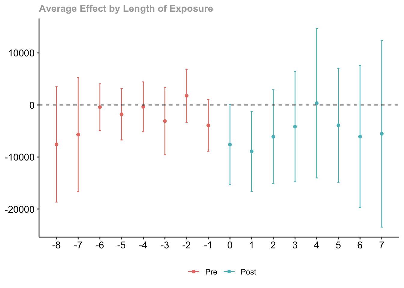
  # part d
  occ_overall <- aggte(occ_res, type="group")
  summary(occ_overall)
Call:
aggte(MP = occ_res, type = "group")

Reference: Callaway, Brantly and Pedro H.C. Sant'Anna.  "Difference-in-Differences with Multiple Time Periods." Journal of Econometrics, Vol. 225, No. 2, pp. 200-230, 2021. <https://doi.org/10.1016/j.jeconom.2020.12.001>, <https://arxiv.org/abs/1803.09015>


Overall summary of ATT's based on group/cohort aggregation:
       ATT    Std. Error     [ 95%  Conf. Int.]
 -7873.709      2280.252  -12342.92   -3404.498 *


Group Effects:
 Group    Estimate Std. Error [95% Simult.  Conf. Band]
  1986  -7202.2226   5471.742     -19171.48    4767.038
  1987   -718.3913   6853.787     -15710.83   14274.050
  1988   1278.5603   6195.673     -12274.28   14831.398
  1990 -14103.4696   4109.816     -23093.56   -5113.379 *
  1991  -1181.1987   7776.333     -18191.68   15829.282
  1992 -19746.4715   4435.389     -29448.74  -10044.200 *
  1993 -27091.4909   5931.060     -40065.49  -14117.487 *
---
Signif. codes: `*' confidence band does not cover 0

Control Group:  Never Treated,  Anticipation Periods:  1
Estimation Method: Doubly Robust- What additional assumptions (with respect to occupation) do you need to make in order to rationalize this approach?